Talent.net data model

To help describe the Talent.net data model, we’ve created a small sample graph, as shown in Figure 5-1, which we’ll use throughout this section to illustrate the Cypher queries behind the main Talent.net use cases.

The sample graph shown here has just two companies, each with several employees. An employee is connected to his employer by a WORKS_FOR relationship. Each employee is INTERESTED_IN one or more topics, and has WORKED_ON one or more projects. Occasionally, employees from different companies work on the same project.

This structure addresses two important use cases:

• Given a user, infer social relations—that is, identify their professional social network—based on shared interests and skills.

• Given a user, recommend someone that they have worked with, or who has worked with people they have worked with, who has a particular skill.

The first use case helps build communities around shared interests. The second helps identify people to fill specific project roles.

Figure 5-1. Sample of the Talent.net social network

Inferring social relations

Talent.net’s graph allows it to infer a user’s professional social network by finding people who share that user’s interests. The strength of the recommendation depends on the number of shared interests. If Sarah is interested in Java, graphs, and REST, Ben in graphs and REST, and Charlie in graphs, cars, and medicine, then there is a likely tie between Sarah and Ben based on their mutual interest in graphs and REST, and another tie between Sarah and Charlie based on their mutual interest in graphs, with the tie between Sarah and Ben stronger than the one between Sarah and Charlie (two shared interests versus one).

Figure 5-2 shows the pattern representing colleagues who share a user’s interests. The subject node refers to the subject of the query (in the preceding example, this is Sarah). This node can be looked up in an index. The remaining nodes will be discovered once the pattern is anchored to the subject node and then flexed around the graph.

The Cypher to implement this query is shown here:

MATCH  (subject:User {name:{name}})
MATCH  (subject)-[:WORKS_FOR]->(company:Company)<-[:WORKS_FOR]-(person:User),
       (subject)-[:INTERESTED_IN]->(interest)<-[:INTERESTED_IN]-(person:User)
RETURN person.name AS name,
       count(interest) AS score,
       collect(interest.name) AS interests
ORDER BY score DESC

Figure 5-2. Pattern to find colleagues who share a user’s interests

The query works as follows:

• The first MATCH finds the subject (here, Sarah) in the nodes labeled User and assigns the result to the subject identifier.

• The second MATCH then matches this User with people who work for the same company, and who share one or more of their interests. If the subject of the query is Sarah, who works for Acme, then in the case of Ben, MATCH will match twice: Ben works for Acme, and is interested in graphs (first match), and REST (second match). In the case of Charlie, it will match once: Charlie works for Acme, and is interested in graphs.

• RETURN creates a projection of the matched data. For each matched colleague, we extract their name, count the number of interests they have in common with the subject of the query (aliasing this result as score), and, using collect, create a comma-separated list of these mutual interests. Where a person has multiple matches, as does Ben in our example, count and collect aggregate their matches into a single row in the returned results. (In fact, both count and collect can perform this aggregating function independently of one another.)

• Finally, we order the results based on each colleague’s score, highest first.

Running this query against our sample graph, with Sarah as the subject, yields the following results:

+---------------------------------------+
| name      | score | interests         |
+---------------------------------------+
| "Ben"     | 2     | ["Graphs","REST"] |
| "Charlie" | 1     | ["Graphs"]        |
+---------------------------------------+
2 rows

Figure 5-3 shows the portion of the graph that was matched to generate these results.

Figure 5-3. Colleagues who share Sarah’s interests

Notice that this query only finds people who work for the same company as Sarah. If we want to extend the search to find people who work for other companies, we need to modify the query slightly:

MATCH  (subject:User {name:{name}})
MATCH  (subject)-[:INTERESTED_IN]->(interest:Topic)
         <-[:INTERESTED_IN]-(person:User),
       (person)-[:WORKS_FOR]->(company:Company)
RETURN person.name AS name,
       company.name AS company,
       count(interest) AS score,
       collect(interest.name) AS interests
ORDER BY score DESC

The changes are as follows:

• In the MATCH clause, we no longer require matched persons to work for the same company as the subject of the query. (We do, however, still capture the company with which a matched person is associated, because we want to return this information in the results.)

• In the RETURN clause we now include the company details for each matched person.

Running this query against our sample data returns the following results:

+---------------------------------------------------------------+
| name      | company        | score | interests                |
+---------------------------------------------------------------+
| "Arnold"  | "Startup, Ltd" | 3     | ["Java","Graphs","REST"] |
| "Ben"     | "Acme, Inc"    | 2     | ["Graphs","REST"]        |
| "Gordon"  | "Startup, Ltd" | 1     | ["Graphs"]               |
| "Charlie" | "Acme, Inc"    | 1     | ["Graphs"]               |
+---------------------------------------------------------------+
4 rows

Figure 5-4 shows the portion of the graph that was matched to generate these results.

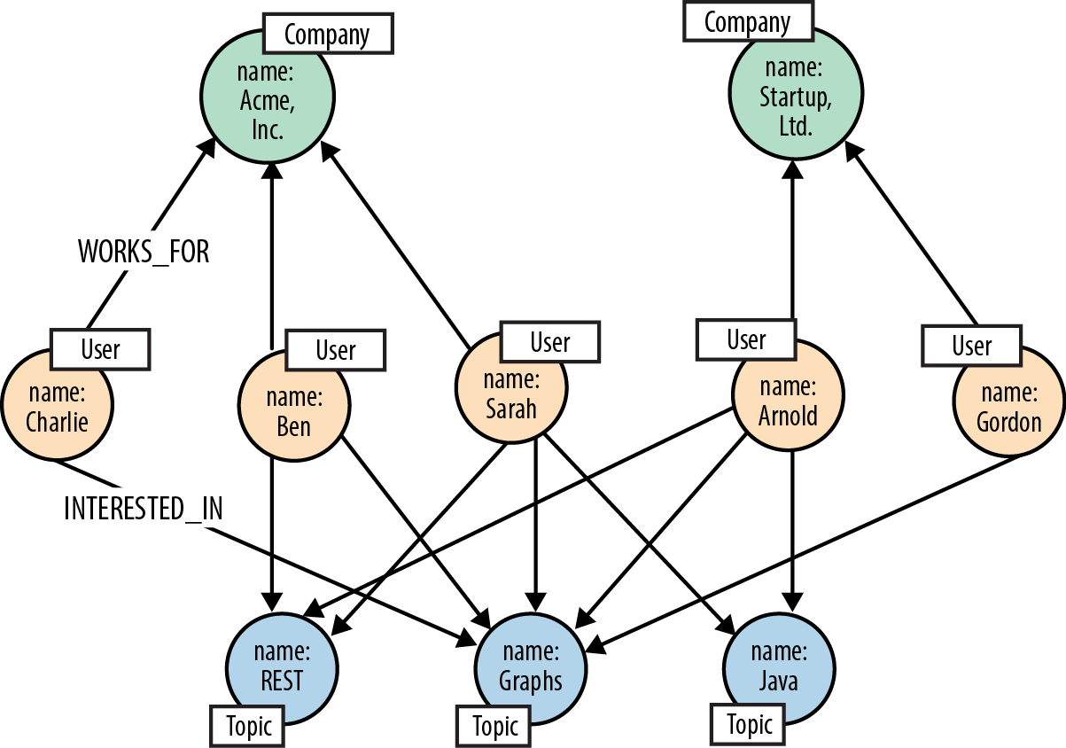
Figure 5-4. People who share Sarah’s interests

Although Ben and Charlie still feature in the results, it turns out that Arnold, who works for Startup, Ltd., has most in common with Sarah: three topics compared to Ben’s two and Charlie’s one.

Finding colleagues with particular interests

In the second Talent.net use case, we turn from inferring social relations based on shared interests to finding individuals who have a particular skillset, and who have either worked with the person who is the subject of the query, or worked with people who have worked with the subject. By applying the graph in this manner we can find individuals to staff project roles based on their social ties to people we trust—or at least with whom we have worked.

The social ties in question arise from individuals having worked on the same project. Contrast this with the previous use case, where the social ties were inferred based on shared interests. If people have worked on the same project, we infer a social tie. The projects, then, form intermediate nodes that bind two or more people together. In other words, a project is an instance of collaboration that has brought several people into contact with one another. Anyone we discover in this fashion is a candidate for including in our results—as long as they possess the interests or skills we are looking for.

Here’s a Cypher query that finds colleagues, and colleagues-of-colleagues, who have one or more particular interests:

MATCH (subject:User {name:{name}})
MATCH p=(subject)-[:WORKED_ON]->(:Project)-[:WORKED_ON*0..2]-(:Project)
        <-[:WORKED_ON]-(person:User)-[:INTERESTED_IN]->(interest:Topic)
WHERE person<>subject AND interest.name IN {interests}
WITH person, interest, min(length(p)) as pathLength
ORDER BY interest.name
RETURN person.name AS name,
       count(interest) AS score,
       collect(interest.name) AS interests,
       ((pathLength - 1)/2) AS distance
ORDER BY score DESC
LIMIT {resultLimit}

This is quite a complex query. Let’s break it down little and look at each part in more detail:

• The first MATCH finds the subject of the query in the nodes labeled User and assigns the result to the subject identifier.

• The second MATCH finds people who are connected to the subject by way of having worked on the same project, or having worked on the same project as people who have worked with the subject. For each person we match, we capture his interests. This match is then further refined by the WHERE clause, which excludes nodes that match the subject of the query, and ensures that we only match people who are interested in the things we care about. For each successful match, we assign the entire path of the match—that is, the path that extends from the subject of the query all the way through the matched person to his interest—to the identifier p. We’ll look at this MATCH clause in more detail shortly.

• WITH pipes the results to the RETURN clause, filtering out redundant paths as it does so. Redundant paths are present in the results at this point because colleagues and colleagues-of-colleagues are often reachable through different paths, some longer than others. We want to filter these longer paths out. That’s exactly what the WITH clause does. The WITH clause emits triples comprising a person, an interest, and the length of the path from the subject of the query through the person to his interest. Given that any particular person/interest combination may appear more than once in the results, but with different path lengths, we want to aggregate these multiple lines by collapsing them to a triple containing only the shortest path, which we do using min(length(p)) as pathLength.

• RETURN creates a projection of the data, performing more aggregation as it does so. The data piped by the WITH clause to RETURN contains one entry per person per interest. If a person matches two of the supplied interests, there will be two separate data entries. We aggregate these entries using count and collect: count to create an overall score for a person, collect to create a comma-separated list of matched interests for that person. As part of the results, we also calculate how far the matched person is from the subject of the query. We do this by taking the pathLength for that person, subtracting one (for the INTERESTED_IN relationship at the end of the path), and then dividing by two (because the person is separated from the subject by pairs of WORKED_ON relationships). Finally, we order the results based on score, highest score first, and limit them according to a resultLimit parameter supplied by the query’s client.

The second MATCH clause in the preceding query uses a variable-length path, [:WORKED_ON*0..2], as part of a larger pattern to match people who have worked directly with the subject of the query, as well as people who have worked on the same project as people who have worked with the subject. Because each person is separated from the subject of the query by one or two pairs of WORKED_ON relationships, Talent.net could have written this portion of the query as MATCH p=(subject)-[:WORKED_ON*2..4]-(person)-[:INTERESTED_IN]->(interest), with a variable-length path of between two and four WORKED_ON relationships. However, long variable-length paths can be relatively inefficient. When writing such queries, it is advisable to restrict variable-length paths to as narrow a scope as possible. To increase the performance of the query, Talent.net uses a fixed-length outgoing WORKED_ON relationship that extends from the subject to her first project, and another fixed-length WORKED_ON relationship that connects the matched person to a project, with a smaller variable-length path in between.

Running this query against our sample graph, and again taking Sarah as the subject of the query, if we look for colleagues and colleagues-of-colleagues who have interests in Java, travel, or medicine, we get the following results:

+--------------------------------------------------+
| name      | score | interests         | distance |
+--------------------------------------------------+
| "Arnold"  | 2     | ["Java","Travel"] | 2        |
| "Charlie" | 1     | ["Medicine"]      | 1        |
+--------------------------------------------------+
2 rows

Note that the results are ordered by score, not distance. Arnold has two out of the three interests, and therefore scores higher than Charlie, who only has one, even though he is at two removes from Sarah, whereas Charlie has worked directly with Sarah.

Figure 5-5 shows the portion of the graph that was traversed and matched to generate these results.

Figure 5-5. Finding people with particular interests

Let’s take a moment to understand how this query executes in more detail. Figure 5-6 shows three stages in the execution of the query. (For visual clarity we’ve removed labels and emphasized the important property values.) The first stage shows each of the paths as they are matched by the MATCH and WHERE clauses. As we can see, there is one redundant path: Charlie is matched directly, through Next Gen Platform, but also indirectly, by way of Quantum Leap and Emily. The second stage represents the filtering that takes place in the WITH clause. Here we emit triples comprising the matched person, the matched interest, and the length of the shortest path from the subject through the matched person to her interest. The third stage represents the RETURN clause, wherein we aggregate the results on behalf of each matched person, and calculate her score and distance from the subject.

Figure 5-6. Query pipeline

Adding WORKED_WITH relationships

The query for finding colleagues and colleagues-of-colleagues with particular interests is the one most frequently executed on Talent.net’s site, and the success of the site depends in large part on its performance. The query uses pairs of WORKED_ON relationships (for example, ('Sarah')-[:WORKED_ON]->('Next Gen Platform')<-[:WORKED_ON]-('Charlie')) to infer that users have worked with one another. Although reasonably performant, this is nonetheless inefficient, because it requires traversing two explicit relationships to infer the presence of a single implicit relationship.

To eliminate this inefficiency, Talent.net decided to precompute a new kind of relationship, WORKED_WITH, thereby enriching the graph with shortcuts for these performance-critical access patterns. As we discussed in “Iterative and Incremental Development”, it’s quite common to optimize graph access by adding a direct relationship between two nodes that would otherwise be connected only by way of intermediaries.

In terms of the Talent.net domain, WORKED_WITH is a bidirectional relationship. In the graph, however, it is implemented using a unidirectional relationship. Although a relationship’s direction can often add useful semantics to its definition, in this instance the direction is meaningless. This isn’t a significant issue, so long as queries that operate with WORKED_WITH relationships ignore the relationship direction.

Calculating a user’s WORKED_WITH relationships and adding them to the graph isn’t difficult, nor is it particularly expensive in terms of resource consumption. It can, however, add milliseconds to any end-user interactions that update a user’s profile with new project information, so Talent.net has decided to perform this operation asynchronously to end-user activities. Whenever a user changes his project history, Talent.net adds a job to a queue. This job recalculates the user’s WORKED_WITH relationships. A single writer thread polls this queue and executes the jobs using the following Cypher statement:

MATCH (subject:User {name:{name}})
MATCH (subject)-[:WORKED_ON]->()<-[:WORKED_ON]-(person:User)
WHERE NOT((subject)-[:WORKED_WITH]-(person))
WITH DISTINCT subject, person
CREATE UNIQUE (subject)-[:WORKED_WITH]-(person)
RETURN subject.name AS startName, person.name AS endName

Figure 5-7 shows what our sample graph looks like once it has been enriched with WORKED_WITH relationships.

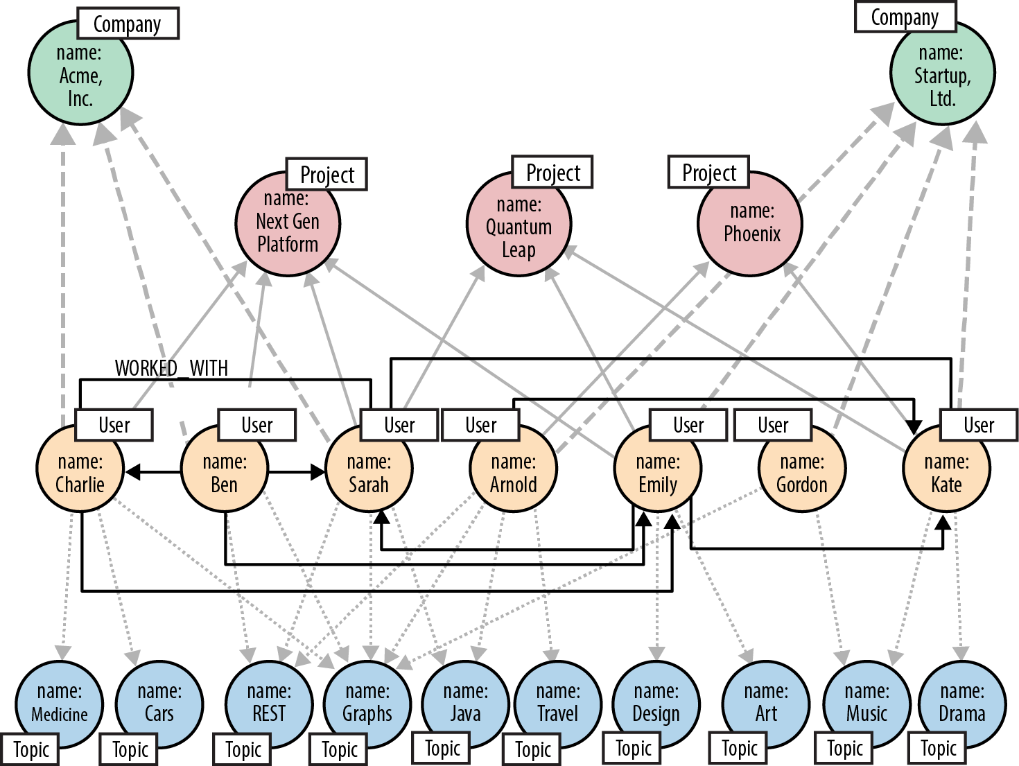
Figure 5-7. Talent.net graph enriched with WORKED_WITH relationships

Using the enriched graph, Talent.net now finds colleagues and colleagues-of-colleagues with particular interests using a slightly simpler version of the query we looked at earlier:

MATCH (subject:User {name:{name}})
MATCH p=(subject)-[:WORKED_WITH*0..1]-(:Person)-[:WORKED_WITH]-(person:User)
        -[:INTERESTED_IN]->(interest:Topic)
WHERE person<>subject AND interest.name IN {interests}
WITH person, interest, min(length(p)) as pathLength
RETURN person.name AS name,
       count(interest) AS score,
       collect(interest.name) AS interests,
       (pathLength - 1) AS distance
ORDER BY score DESC
LIMIT {resultLimit}

TeleGraph data model

Figure 5-8 shows a sample of the TeleGraph data model. (For clarity, labels are presented at the top of each set of nodes once only, rather than being attached to every node. In the real data, all nodes have at least one label.)

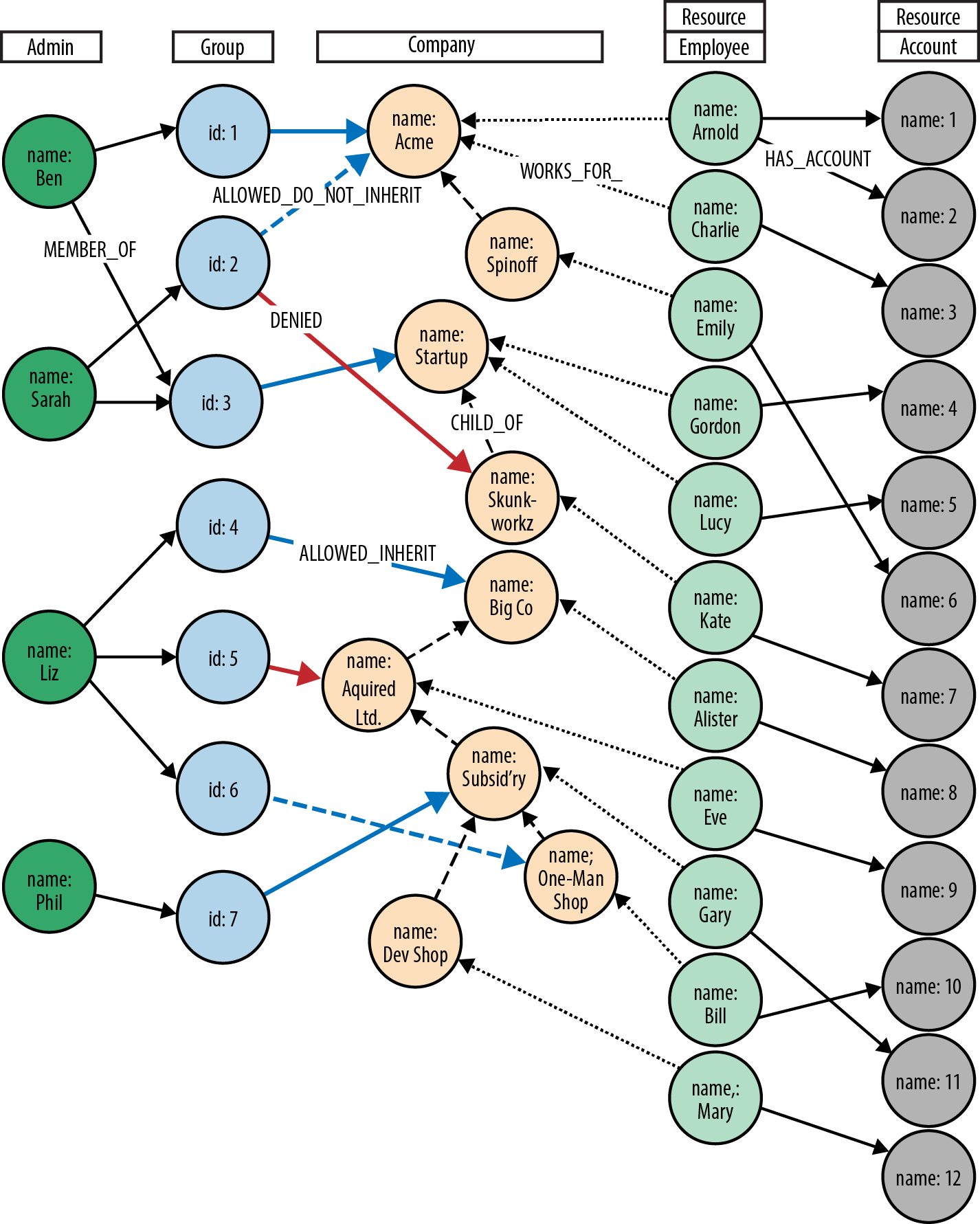
Figure 5-8. Access control graph

This model comprises two hierarchies. In the first hierarchy, administrators within each customer organization are assigned to groups. These groups are then accorded various permissions against that organization’s organizational structure:

• ALLOWED_INHERIT connects an administrator group to an organizational unit, thereby allowing administrators within that group to manage the organizational unit. This permission is inherited by children of the parent organizational unit. We see an example of inherited permissions in the TeleGraph example data model in the relationships between Group 1 and Acme, and the child of Acme, Spinoff. Group 1 is connected to Acme using an ALLOWED_INHERIT relationship. Ben, as a member of Group 1, can manage employees both of Acme and Spinoff thanks to this ALLOWED_INHERIT relationship.

• ALLOWED_DO_NOT_INHERIT connects an administrator group to an organizational unit in a way that allows administrators within that group to manage the organizational unit, but not any of its children. Sarah, as a member of Group 2, can administer Acme, but not its child Spinoff, because Group 2 is connected to Acme by an ALLOWED_DO_NOT_INHERIT relationship, not an ALLOWED_INHERIT relationship.

• DENIED forbids administrators from accessing an organizational unit. This permission is inherited by children of the parent organizational unit. In the TeleGraph diagram, this is best illustrated by Liz and her permissions with respect to Big Co, Acquired Ltd, Subsidiary, and One-Map Shop. As a result of her membership of Group 4 and its ALLOWED_INHERIT permission on Big Co, Liz can manage Big Co. But despite this being an inheritable relationship, Liz cannot manage Acquired Ltd or Subsidiary because Group 5, of which Liz is a member, is DENIED access to Acquired Ltd and its children (which includes Subsidiary). Liz can, however, manage One-Map Shop, thanks to an ALLOWED_DO_NOT_INHERIT permission granted to Group 6, the last group to which Liz belongs.

DENIED takes precedence over ALLOWED_INHERIT, but is subordinate to ALLOWED_DO_NOT_INHERIT. Therefore, if an administrator is connected to a company by way of ALLOWED_DO_NOT_INHERIT and DENIED, ALLOWED_DO_NOT_INHERIT prevails.

Finding all accessible resources for an administrator

The TeleGraph application uses many different Cypher queries. We’ll look at just a few of them here.

First up is the ability to find all the resources an administrator can access. Whenever an onsite administrator logs in to the system, he is presented with a list of all the employees and employee accounts he can administer. This list is generated based on the results returned from the following query:

MATCH (admin:Admin {name:{adminName}})
MATCH paths=(admin)-[:MEMBER_OF]->(:Group)-[:ALLOWED_INHERIT]->(:Company)
        <-[:CHILD_OF*0..3]-(company:Company)<-[:WORKS_FOR]-(employee:Employee)
        -[:HAS_ACCOUNT]->(account:Account)
WHERE NOT ((admin)-[:MEMBER_OF]->(:Group)
            -[:DENIED]->(:Company)<-[:CHILD_OF*0..3]-(company))
RETURN employee.name AS employee, account.name AS account
UNION
MATCH (admin:Admin {name:{adminName}})
MATCH paths=(admin)-[:MEMBER_OF]->(:Group)-[:ALLOWED_DO_NOT_INHERIT]->(:Company)
        <-[:WORKS_FOR]-(employee:Employee)-[:HAS_ACCOUNT]->(account:Account)
RETURN employee.name AS employee, account.name AS account

Like all the other queries we’ll be looking at in this section, this query comprises two separate queries joined by a UNION operator. The query before the UNION operator handles ALLOWED_INHERIT relationships qualified by any DENIED relationships. The query following the UNION operator handles any ALLOWED_DO_NOT_INHERIT permissions. This pattern, ALLOWED_INHERIT minus DENIED, followed by ALLOWED_DO_NOT_INHERIT, is repeated in all of the access control example queries that we’ll be looking at.

The first query here, the one before the UNION operator, can be broken down as follows:

• The first MATCH selects the logged-in administrator from the nodes labeled Administrator, and binds the result to the admin identifier.

• MATCH matches all the groups to which this administrator belongs, and from these groups, all the parent companies connected by way of an ALLOWED_INHERIT relationship. The MATCH then uses a variable-length path ([:CHILD_OF*0..3]) to discover children of these parent companies, and thereafter the employees and accounts associated with all matched companies (whether parent company or child). At this point, the query has matched all companies, employees, and accounts accessible by way of ALLOWED_INHERIT relationships.

• WHERE eliminates matches whose company, or parent companies, are connected by way of a DENIED relationship to the administrator’s groups. This WHERE clause is invoked for each match. If there is a DENIED relationship anywhere between the admin node and the company node bound by the match, that match is eliminated.

• RETURN creates a projection of the matched data in the form of a list of employee names and accounts.

The second query here, following the UNION operator, is a little simpler:

• The first MATCH selects the logged-in administrator from the nodes labeled Administrator, and binds the result to the admin identifier.

• The second MATCH simply matches companies (plus employees and accounts) that are directly connected to an administrator’s groups by way of an ALLOWED_DO_NOT_INHERIT relationship.

The UNION operator joins the results of these two queries together, eliminating any duplicates. Note that the RETURN clause in each query must contain the same projection of the results. In other words, the column names in the two result sets must match.

Figure 5-9 shows how this query matches all accessible resources for Sarah in the sample TeleGraph graph. Note that, because of the DENIED relationship from Group 2 to Skunkworkz, Sarah cannot administer Kate and Account 7.

Figure 5-9. Finding all accessible resources for a user

Determining whether an administrator has access to a resource

The query we’ve just looked at returned a list of employees and accounts an administrator can manage. In a web application, each of these resources (employee, account) is accessible through its own URI. Given a friendly URI (e.g., http://TeleGraph/accounts/5436), what’s to stop someone from hacking a URI and gaining illegal access to an account?

What’s needed is a query that will determine whether an administrator has access to a specific resource. This is that query:

MATCH (admin:Admin {name:{adminName}}),
      (company:Company)-[:WORKS_FOR|HAS_ACCOUNT*1..2]
        -(resource:Resource {name:{resourceName}})
MATCH p=(admin)-[:MEMBER_OF]->(:Group)-[:ALLOWED_INHERIT]->(:Company)
        <-[:CHILD_OF*0..3]-(company)
WHERE NOT ((admin)-[:MEMBER_OF]->(:Group)-[:DENIED]->(:Company)
            <-[:CHILD_OF*0..3]-(company))
RETURN count(p) AS accessCount
UNION
MATCH (admin:Admin {name:{adminName}}),
      (company:Company)-[:WORKS_FOR|HAS_ACCOUNT*1..2]
        -(resource:Resource {name:{resourceName}})
MATCH p=(admin)-[:MEMBER_OF]->()-[:ALLOWED_DO_NOT_INHERIT]->(company)
RETURN count(p) AS accessCount

This query works by determining whether an administrator has access to the company to which an employee or an account belongs. Given an employee or account, we need to determine the company with which this resource is associated, and then work out whether the administrator has access to that company.

How do we identify the company to which an employee or account belongs? By labelling both as Resource (as well as either Company or Account). An employee is connected to a company resource by a WORKS_FOR relationship. An account is associated with a company by way of an employee. HAS_ACCOUNT connects the employee to the account. WORKS_FOR then connects this employee to the company. In other words, an employee is one hop away from a company, whereas an account is two hops away from a company.

With that bit of insight, we can see that this resource authorization check is similar to the query for finding all companies, employees, and accounts—only with several small differences:

• The first MATCH findz the company to which an employee or account belongs. It uses Cypher’s OR operator, |, to match both WORKS_FOR and HAS_ACCOUNT relationships at depth one or two.

• The WHERE clause in the query before the UNION operator eliminates matches where the company in question is connected to one of the administrator’s groups by way of a DENIED relationship.

• The RETURN clauses for the queries before and after the UNION operator return a count of the number of matches. For an administrator to have access to a resource, one or both of these accessCount values must be greater than 0.

Because the UNION operator eliminates duplicate results, the overall result set for this query can contain either one or two values. The client-side algorithm for determining whether an administrator has access to a resource can be expressed easily in Java:

private boolean isAuthorized( Result result )
{
    Iterator<Long> accessCountIterator = result.columnAs( "accessCount" );
    while ( accessCountIterator.hasNext() )
    {
        if (accessCountIterator.next() > 0L)
        {
            return true;
        }
    }
    return false;
}

Finding administrators for an account

The previous two queries represent “top-down” views of the graph. The last TeleGraph query we’ll discuss here provides a “bottom-up” view of the data. Given a resource—an employee or account—who can manage it? Here’s the query:

MATCH (resource:Resource {name:{resourceName}})
MATCH p=(resource)-[:WORKS_FOR|HAS_ACCOUNT*1..2]-(company:Company)
        -[:CHILD_OF*0..3]->()<-[:ALLOWED_INHERIT]-()<-[:MEMBER_OF]-(admin:Admin)
WHERE NOT ((admin)-[:MEMBER_OF]->(:Group)-[:DENIED]->(:Company)
            <-[:CHILD_OF*0..3]-(company))
RETURN admin.name AS admin
UNION
MATCH (resource:Resource {name:{resourceName}})
MATCH p=(resource)-[:WORKS_FOR|HAS_ACCOUNT*1..2]-(company:Company)
        <-[:ALLOWED_DO_NOT_INHERIT]-(:Group)<-[:MEMBER_OF]-(admin:Admin)
RETURN admin.name AS admin

As before, the query consists of two independent queries joined by a UNION operator. Of particular note are the following clauses:

• The first MATCH clause uses a Resource label, which allows it to identify both employees and accounts.

• The second MATCH clauses contain a variable-length path expression that uses the | operator to specify a path that is one or two relationships deep, and whose relationship types comprise WORKS_FOR or HAS_ACCOUNT. This expression accommodates the fact that the subject of the query may be either an employee or an account.

Figure 5-10 shows the portions of the graph matched by the query when asked to find the administrators for Account 10.

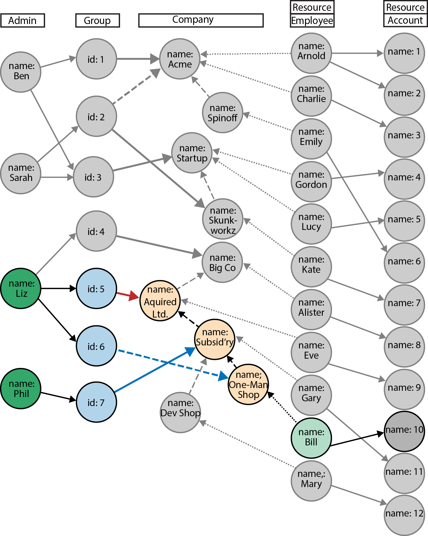
Figure 5-10. Finding an administrator for a specific account

Global Post data model

Figure 5-11 shows a simple example of the Global Post parcel network. The network comprises parcel centers, which are connected to delivery bases, each of which covers several delivery areas. These delivery areas, in turn, are subdivided into delivery segments covering many delivery units. There are around 25 national parcel centers and roughly 2 million delivery units (corresponding to postal or zip codes).

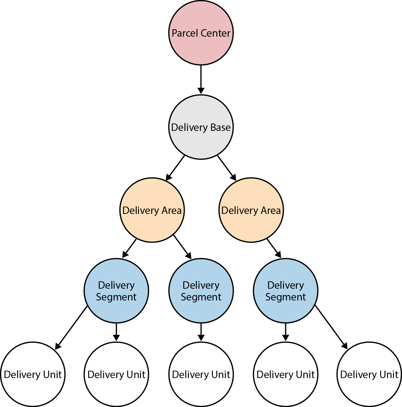
Figure 5-11. Elements in the Global Post network

Over time, the delivery routes change. Figures 5-12, 5-13, and 5-14 show three distinct delivery periods. For any given period, there is at most one route between a delivery base and any particular delivery area or segment. In contrast, there are multiple routes between delivery bases and parcel centers throughout the year. For any given point in time, therefore, the lower portions of the graph (the individual subgraphs below each delivery base) comprise simple tree structures, whereas the upper portions of the graph, made up of delivery bases and parcel centers, are more interconnected.

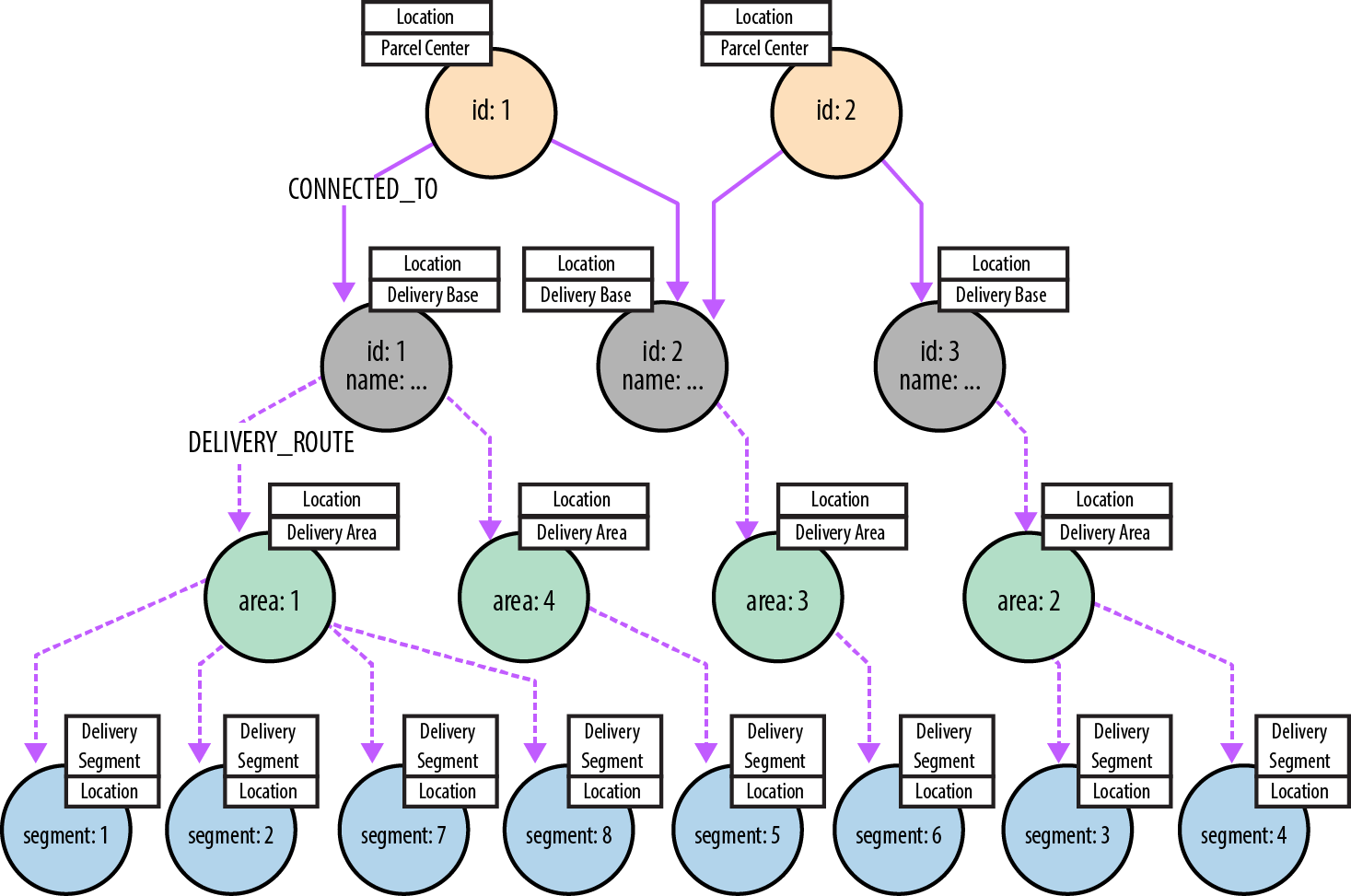
Figure 5-12. Structure of the delivery network for Period 1

Figure 5-13. Structure of the delivery network for Period 2

Figure 5-14. Structure of the delivery network for Period 3

Notice that delivery units are not included in the production data. This is because each delivery unit is always associated with the same delivery segments, irrespective of the period. Because of this invariant, it is possible to index each delivery segment by its many delivery units. To calculate the route to a particular delivery unit, the system need only actually calculate the route to its associated delivery segment, the name of which can be recovered from the index using the delivery unit as a key. This optimization helps both reduce the size of the production graph, and reduce the number of traversals needed to calculate a route.

The production database contains the details of all the different delivery periods. As shown in Figure 5-15, the presence of so many period-specific relationships makes for a densely connected graph.

In the production data, nodes are connected by multiple relationships, each of which is timestamped with a start_date and end_date property. Relationships are of two types: CONNECTED_TO, which connects parcel centers and delivery bases, and DELIVERY_ROUTE, which connects delivery bases to delivery areas, and delivery areas to delivery segments. These two different types of relationships effectively partition the graph into its upper and lower parts, a strategy that provides for very efficient traversals. Figure 5-16 shows three of the timestamped CONNECTED_TO relationships connecting a parcel center to a delivery base.

Figure 5-15. Sample of the Global Post network

Route calculation

As described in the previous section, the CONNECTED_TO and DELIVERY_ROUTE relationships partition the graph into upper and lower parts, with the upper parts made up of complexly connected parcel centers and delivery centers, the lower parts of delivery bases, delivery areas, and delivery segments organized—for any given period—in simple tree structures.

Route calculations involve finding the cheapest route between two locations in the lower portions of the graph. The starting location is typically a delivery segment or delivery area, whereas the end location is always a delivery segment. A delivery segment, as we discussed earlier, is effectively a key for a delivery unit. Irrespective of the start and end locations, the calculated route must go via at least one parcel center in the upper part of the graph.

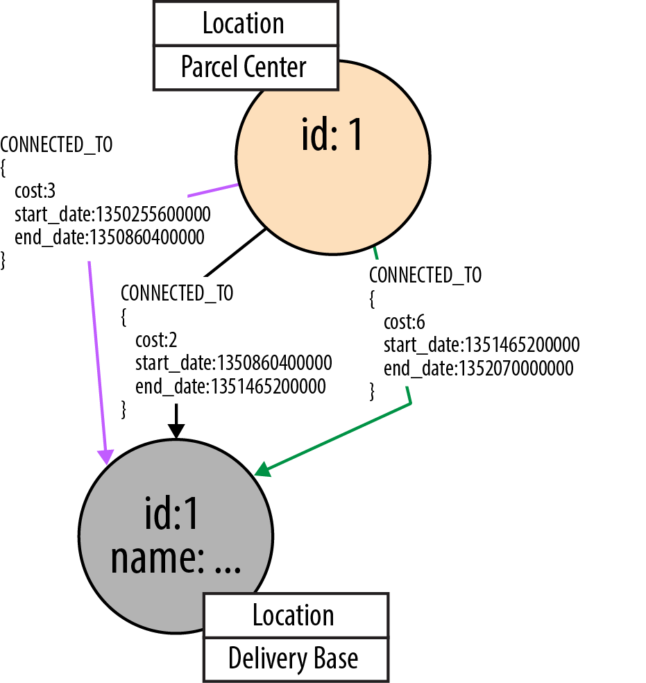
Figure 5-16. Timestamp properties on relationships

In terms of traversing the graph, a calculation can be split into three legs. Legs one and two, shown in Figure 5-17, work their way upward from the start and end locations, respectively, with each terminating at a delivery center. Because there is at most one route between any two elements in the lower portion of the graph for any given delivery period, traversing from one element to the next is simply a matter of finding an incoming DELIVERY ROUTE relationship whose interval timestamps encompass the current delivery period. By following these relationships, the traversals for legs one and two navigate a pair of tree structures rooted at two different delivery centers. These two delivery centers then form the start and end locations for the third leg, which crosses the upper portion of the graph.

Figure 5-17. Shortest path to delivery bases from start and end points

As with legs one and two, the traversal for leg three, as shown in Figure 5-18, looks for relationships—this time, CONNECTED_TO relationships—whose timestamps encompass the current delivery period. Even with this time filtering in place, however, there are, for any given period, potentially several routes between any two delivery centers in the upper portion of the graph. The third leg traversal must, therefore, sum the cost of each route, and select the cheapest, making this a shortest weighted path calculation.

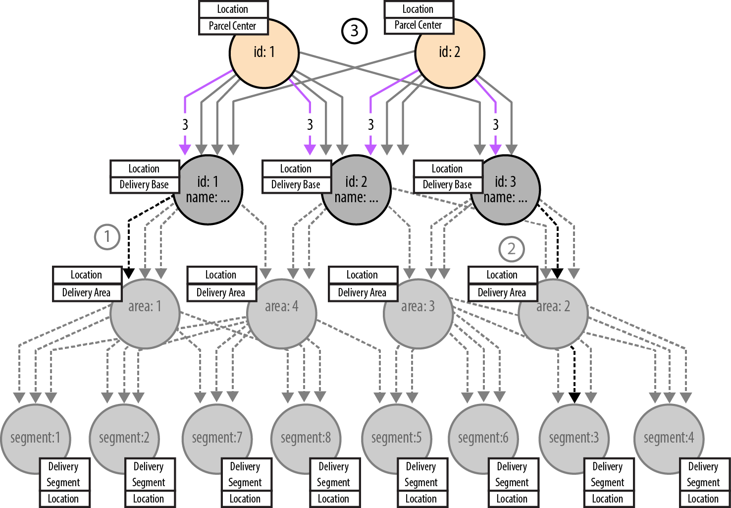
Figure 5-18. Shortest path between delivery bases

To complete the calculation, we need then simply to add the paths for legs one, three, and two, which gives the full path from the start to the end location.

Finding the shortest delivery route using Cypher

The Cypher query to implement the parcel route calculation engine is as follows:

MATCH (s:Location {name:{startLocation}}),
      (e:Location {name:{endLocation}})
MATCH upLeg = (s)<-[:DELIVERY_ROUTE*1..2]-(db1)
WHERE all(r in relationships(upLeg)
          WHERE r.start_date <= {intervalStart}
          AND r.end_date >= {intervalEnd})
WITH  e, upLeg, db1
MATCH downLeg = (db2)-[:DELIVERY_ROUTE*1..2]->(e)
WHERE all(r in relationships(downLeg)
          WHERE r.start_date <= {intervalStart}
          AND r.end_date >= {intervalEnd})
WITH  db1, db2, upLeg, downLeg
MATCH topRoute = (db1)<-[:CONNECTED_TO]-()-[:CONNECTED_TO*1..3]-(db2)
WHERE all(r in relationships(topRoute)
          WHERE r.start_date <= {intervalStart}
          AND r.end_date >= {intervalEnd})
WITH  upLeg, downLeg, topRoute,
      reduce(weight=0, r in relationships(topRoute) | weight+r.cost) AS score
      ORDER BY score ASC
      LIMIT 1
RETURN (nodes(upLeg) + tail(nodes(topRoute)) + tail(nodes(downLeg))) AS n

At first glance, this query appears quite complex. It is, however, made up of four simpler queries joined together with WITH clauses. We’ll look at each of these subqueries in turn.

Here’s the first subquery:

MATCH (s:Location {name:{startLocation}}),
      (e:Location {name:{endLocation}})
MATCH upLeg = (s)<-[:DELIVERY_ROUTE*1..2]-(db1)
WHERE all(r in relationships(upLeg)
          WHERE r.start_date <= {intervalStart}
          AND r.end_date >= {intervalEnd})

This query calculates the first leg of the overall route. It can be broken down as follows:

• The first MATCH finds the start and end locations in the subset of nodes labeled Location, binding them to the s and e identifiers, respectively.

• The second MATCH finds the route from the start location, s, to a delivery base using a directed, variable-length DELIVERY_ROUTE path. This path is then bound to the identifier upLeg. Because delivery bases are always the root nodes of DELIVERY_ROUTE trees, and therefore have no incoming DELIVERY_ROUTE relationships, we can be confident that the db1 node at the end of this variable-length path represents a delivery base and not some other parcel network element.

• WHERE applies additional constraints to the path upLeg, ensuring that we only match DELIVERY_ROUTE relationships whose start_date and end_date properties encompass the supplied delivery period.

The second subquery calculates the second leg of the route, which comprises the path from the end location up to the delivery base whose DELIVERY_ROUTE tree includes that end location as a leaf node. This query is very similar to the first:

WITH  e, upLeg, db1
MATCH downLeg = (db2)-[:DELIVERY_ROUTE*1..2]->(e)
WHERE all(r in relationships(downLeg)
          WHERE r.start_date <= {intervalStart}
          AND r.end_date >= {intervalEnd})

The WITH clause here chains the first subquery to the second, piping the end location and the first leg’s path and delivery base to the second subquery. The second subquery uses only the end location, e, in its MATCH clause; the rest is provided so that it can be piped to subsequent queries.

The third subquery identifies all candidate paths for the third leg of the route—that is, the route between delivery bases db1 and db2—as follows:

WITH  db1, db2, upLeg, downLeg
MATCH topRoute = (db1)<-[:CONNECTED_TO]-()-[:CONNECTED_TO*1..3]-(db2)
WHERE all(r in relationships(topRoute)
          WHERE r.start_date <= {intervalStart}
          AND r.end_date >= {intervalEnd})

This subquery is broken down as follows:

• WITH chains this subquery to the previous one, piping delivery bases db1 and db2 together with the paths identified in legs one and two to the current query.

• MATCH identifies all paths between the first and second leg delivery bases, to a maximum depth of four, and binds them to the topRoute identifier.

• WHERE constrains the topRoute paths to those whose start_date and end_date properties encompass the supplied delivery period.

The fourth and final subquery selects the shortest path for leg three, and then calculates the overall route:

WITH  upLeg, downLeg, topRoute,
      reduce(weight=0, r in relationships(topRoute) | weight+r.cost) AS score
      ORDER BY score ASC
      LIMIT 1
RETURN (nodes(upLeg) + tail(nodes(topRoute)) + tail(nodes(downLeg))) AS n

This subquery works as follows:

• WITH pipes one or more triples, comprising upLeg, downLeg, and topRoute paths, to the current query. There will be one triple for each of the paths matched by the third subquery, with each path being bound to topRoute in successive triples (the paths bound to upLeg and downLeg will stay the same, because the first and second subqueries matched only one path each). Each triple is accompanied by a score for the path bound to topRoute for that triple. This score is calculated using Cypher’s reduce function, which for each triple sums the cost properties on the relationships in the path currently bound to topRoute. The triples are then ordered by this score, lowest first, and then limited to the first triple in the sorted list.

• RETURN sums the nodes in the paths upLeg, topRoute, and downLeg to produce the final results. The tail function drops the first node in each of the paths topRoute and downLeg, because that node will already be present in the preceding path.

Implementing route calculation with the Traversal Framework

The time-critical nature of the route calculation imposes strict demands on the route calculation engine. As long as the individual query latencies are low enough, it’s always possible to scale horizontally for increased throughput. The Cypher-based solution is fast, but with many thousands of parcels entering the network each second, every millisecond impacts the cluster footprint. For this reason, Global Post adopted an alternative approach: calculating routes using Neo4j’s Traversal Framework.

A traversal-based implementation of the route calculation engine must solve two problems: finding the shortest paths, and filtering the paths based on time period. We’ll look at how we filter paths based on time period first.

Traversals should only follow relationships that are valid for the specified delivery period. In other words, as the traversal progresses through the graph, it should be presented with only those relationships whose periods of validity, as defined by their start_date and end_date properties, contain the specified delivery period.

We implement this relationship filtering using a PathExpander. Given a path from a traversal’s start node to the node where it is currently positioned, a PathExpander’s expand() method returns the relationships that can be used to traverse further. This method is called by the Traversal Framework each time the framework advances another node into the graph. If needed, the client can supply some initial state, called the branch state, to the traversal. The expand() method can use (and even change) the supplied branch state in the course of deciding which relationships to return. The route calculator’s ValidPathExpander implementation uses this branch state to supply the delivery period to the expander.

Here’s the code for the ValidPathExpander:

private static class ValidPathExpander implements PathExpander<Interval>
{
  private final RelationshipType relationshipType;
  private final Direction direction;

  private ValidPathExpander( RelationshipType relationshipType,
                             Direction direction )
  {
      this.relationshipType = relationshipType;
      this.direction = direction;
  }

  @Override
  public Iterable<Relationship> expand( Path path,
                                        BranchState<Interval> deliveryInterval )
  {
      List<Relationship> results = new ArrayList<Relationship>();
      for ( Relationship r : path.endNode()
                             .getRelationships( relationshipType, direction ) )
      {
          Interval relationshipInterval = new Interval(
              (Long) r.getProperty( "start_date" ),
              (Long) r.getProperty( "end_date" ) );
          if ( relationshipInterval.contains( deliveryInterval.getState() ) )
          {
              results.add( r );
          }
      }

      return results;
  }
}

The ValidPathExpander’s constructor takes two arguments: a relationshipType and a direction. This allows the expander to be reused for different types of relationships. In the case of the Global Post graph, the expander will be used to filter both CONNECTED_TO and DELIVERY_ROUTE relationships.

The expander’s expand() method takes as parameters the path that extends from the traversal’s start node to the node on which the traversal is currently positioned, and the deliveryInterval branch state as supplied by the client. Each time it is called, expand() iterates the relevant relationships on the current node (the current node is given by path.endNode()). For each relationship, the method then compares the relationship’s interval with the supplied delivery interval. If the relationship’s interval contains the delivery interval, the relationship is added to the results.

Having looked at the ValidPathExpander, we can now turn to the ParcelRouteCalculator itself. This class encapsulates all the logic necessary to calculate a route between the point where a parcel enters the network and the final delivery destination. It employs a similar strategy to the Cypher query we’ve already looked at. That is, it works its way up the graph from both the start node and the end node in two separate traversals, until it finds a delivery base for each leg. It then performs a shortest weighted path search that joins these two delivery bases.

Here’s the beginning of the ParcelRouteCalculator class:

public class ParcelRouteCalculator
{
    private static final PathExpander<Interval> DELIVERY_ROUTE_EXPANDER =
        new ValidPathExpander( withName( "DELIVERY_ROUTE" ),
                               Direction.INCOMING );

    private static final PathExpander<Interval> CONNECTED_TO_EXPANDER =
        new ValidPathExpander( withName( "CONNECTED_TO" ),
                               Direction.BOTH );

    private static final TraversalDescription DELIVERY_BASE_FINDER =
        Traversal.description()
            .depthFirst()
            .evaluator( new Evaluator()
            {
                private final RelationshipType DELIVERY_ROUTE =
                    withName( "DELIVERY_ROUTE");

                @Override
                public Evaluation evaluate( Path path )
                {
                    if ( isDeliveryBase( path ) )
                    {
                        return Evaluation.INCLUDE_AND_PRUNE;
                    }

                    return Evaluation.EXCLUDE_AND_CONTINUE;
                }

                private boolean isDeliveryBase( Path path )
                {
                    return !path.endNode().hasRelationship(
                        DELIVERY_ROUTE, Direction.INCOMING );
                }
            } );

    private static final CostEvaluator<Double> COST_EVALUATOR =
        CommonEvaluators.doubleCostEvaluator( "cost" );
    public static final Label LOCATION = DynamicLabel.label("Location");
    private GraphDatabaseService db;

    public ParcelRouteCalculator( GraphDatabaseService db )
    {
        this.db = db;
    }
    ...
}

Here we define two expanders—one for DELIVERY_ROUTE relationships, another for CONNECTED_TO relationships—and the traversal that will find the two legs of our route. This traversal terminates whenever it encounters a node with no incoming DELIVERY_ROUTE relationships. Because each delivery base is at the root of a delivery route tree, we can infer that a node without any incoming DELIVERY_ROUTE relationships represents a delivery base in our graph.

Each route calculation engine maintains a single instance of this route calculator. This instance is capable of servicing multiple requests. For each route to be calculated, the client calls the calculator’s calculateRoute() method, passing in the names of the start and end points, and the interval for which the route is to be calculated:

public Iterable<Node> calculateRoute( String start,
                                      String end,
                                      Interval interval )
{
    try ( Transaction tx = db.beginTx() )
    {
        TraversalDescription deliveryBaseFinder =
            createDeliveryBaseFinder( interval );

        Path upLeg = findRouteToDeliveryBase( start, deliveryBaseFinder );
        Path downLeg = findRouteToDeliveryBase( end, deliveryBaseFinder );

        Path topRoute = findRouteBetweenDeliveryBases(
            upLeg.endNode(),
            downLeg.endNode(),
            interval );

        Set<Node> routes = combineRoutes(upLeg, downLeg, topRoute);
        tx.success();
        return routes;
    }
}

calculateRoute() first obtains a deliveryBaseFinder for the specified interval, which it then uses to find the routes for the two legs. Next, it finds the route between the delivery bases at the top of each leg, these being the last nodes in each leg’s path. Finally, it combines these routes to generate the final results.

The createDeliveryBaseFinder() helper method creates a traversal description configured with the supplied interval:

private TraversalDescription createDeliveryBaseFinder( Interval interval )
{
    return DELIVERY_BASE_FINDER.expand( DELIVERY_ROUTE_EXPANDER,
        new InitialBranchState.State<>( interval, interval ) );
}

This traversal description is built by expanding the ParcelRouteCalculator’s static DELIVERY_BASE_FINDER traversal description using the DELIVERY_ROUTE_EXPANDER. The branch state for the expander is initialized at this point with the interval supplied by the client. This enables us to use the same base traversal description instance (DELIVERY_BASE_FINDER) for multiple requests. This base description is expanded and parameterized for each request.

Properly configured with an interval, the traversal description is then supplied to findRouteToDeliveryBase(), which looks up a starting node in the location index, and then executes the traversal:

private Path findRouteToDeliveryBase( String startPosition,
                                      TraversalDescription deliveryBaseFinder )
{
  Node startNode = IteratorUtil.single(
	    db.findNodesByLabelAndProperty(LOCATION, "name", startPosition));
  return deliveryBaseFinder.traverse( startNode ).iterator().next();
}

That’s the two legs taken care of. The last part of the calculation requires us to find the shortest path between the delivery bases at the top of each of the legs. calculateRoute() takes the last node from each leg’s path, and supplies these two nodes together with the client-supplied interval to findRouteBetweenDeliveryBases(). Here’s the implementation of findRouteBetweenDeliveryBases():

private Path findRouteBetweenDeliveryBases( Node deliveryBase1,
                                            Node deliveryBase2,
                                            Interval interval )
{
    PathFinder<WeightedPath> routeBetweenDeliveryBasesFinder =
        GraphAlgoFactory.dijkstra(
            CONNECTED_TO_EXPANDER,
            new InitialBranchState.State<>( interval, interval ),
            COST_EVALUATOR );

    return routeBetweenDeliveryBasesFinder
        .findSinglePath( deliveryBase1, deliveryBase2 );
}

Rather than use a traversal description to find the shortest route between two nodes, this method uses a shortest weighted path algorithm from Neo4j’s graph algorithm library—in this instance, we’re using the Dijkstra algorithm (see “Path-Finding with Dijkstra’s Algorithm” for more details on the Dijkstra algorithm). This algorithm is configured with ParcelRouteCalculator’s static CONNECTED_TO_EXPANDER, which in turn is initialized with the client-supplied branch state interval. The algorithm is also configured with a cost evaluator (another static member), which simply identifies the property on a relationship representing that relationship’s weight or cost. A call to findSinglePath on the Dijkstra path finder returns the shortest path between the two delivery bases.

That’s the hard work done. All that remains is to join these routes to form the final results. This is relatively straightforward, the only wrinkle being that the down leg’s path must be reversed before being added to the results (the leg was calculated from final destination upward, whereas it should appear in the results delivery base downward):

private Set<Node> combineRoutes( Path upLeg,
                                 Path downLeg,
                                 Path topRoute )
{
    LinkedHashSet<Node> results = new LinkedHashSet<>();
    results.addAll( IteratorUtil.asCollection( upLeg.nodes() ));
    results.addAll( IteratorUtil.asCollection( topRoute.nodes() ));
    results.addAll( IteratorUtil.asCollection( downLeg.reverseNodes() ));
    return results;
}