
Chapter 4
Multi-homing for a Green Downlink
In a heterogeneous wireless medium, downlink multi-homing radio resource allocation can save power for network operators. In this context, two application scenarios can be distinguished. In the first scenario, the MT aggregates the offered radio resources from different networks to support a single (data hungry) application, while in the second scenario, the MT runs different applications using the radio resources assigned to different radio interfaces. In this chapter, we discuss the challenging issues associated with each application scenario. Two radio resource allocation mechanisms are presented to address the corresponding challenges.
4.1 Introduction
The increasing demand for wireless communication services and the wide deployment of wireless communication infrastructures have led to high power consumption in the wireless access networks. Due to financial and environmental concerns, wireless network service providers have shown a growing interest in deploying power-efficient wireless communication infrastructures. Given today's heterogeneous wireless medium with overlapped coverage from different networks and the multi-homing capabilities of MTs, green multi-homing radio resource allocation in the downlink can lead to power saving for the network operators. Green multi-homing techniques can be adopted in two application scenarios. The first scenario aggregates the offered radio resources from different networks to support in the downlink a single (data or video) call using multiple threads at the application layer. The second scenario assumes different applications running at the MT, and it can be supported using different radio resources from different networks. For instance, the MT can make a video call using the radio resources offered to one radio interface while performing a data call using the radio resources offered at another radio interface.
For the first application scenario, several networks with overlapped coverage can cooperate in allocating their radio resources to MTs to satisfy the required service quality at reduced power consumption. Network cooperative (multi-homing) radio resource allocation can lead to a higher power saving than the single-network (non-cooperative) mechanisms, due to the diversity in the wireless channels between MTs and different BSs and in the available resources at the BSs of different networks. However, the existing cooperative networking mechanisms suffer from several limitations. First, there exists an implicit assumption that different networks are willing to cooperate unconditionally to reduce the total power consumption within a certain geographical region (e.g. [32, 33] and [36]). This assumption is valid in the case that all networks are operated by the same service provider. In a cooperative networking scenario, the total (sum) power consumption can be reduced at the cost of increasing the power consumption for one operator, as compared with the non-cooperative case. Hence, when different networks are operated by different service providers, cooperation is appropriate only if it results in mutual benefit (i.e. power saving) for all the networks. The second limitation with existing cooperative networking mechanisms is that they adopt only power allocation techniques, assuming some fixed bandwidth allocation (e.g. [33] and [133]). Such an approach focuses mainly on exploiting only one dimension in the heterogeneous wireless medium, which is the diverse fading channels and propagation losses among MTs and BSs of different networks. Another dimension that should be accounted for is the disparity in the available bandwidth at BSs of different networks. Therefore, joint bandwidth and power allocation (within the framework described in Chapter 3) should be investigated for improved power saving in such a networking environment. Finally, the existing mechanisms rely on a central manager for resource allocation (e.g. [134] and references therein). Such mechanisms are useful in a single-operator scenario; however, they are infeasible in a multi-operator scenario due to the absence of a central entity. Instead, decentralized mechanisms that enable coordinated resource allocation among different networks are required.
On the other hand, for the second application scenario, when two radio interfaces operate simultaneously using different radio technologies with adjacent frequency bands (e.g. LTE and WiFi), the OOB radiations of the transmitting radio (on the uplink) leak on the receiving radio (on the downlink), and hence, the MT suffers from IDC interference as discussed in Chapter 3. Without appropriate consideration of the IDC interference in the radio resource allocation, network operators will be subject to high power consumption in the downlink to overcome the interference of the MT uplink transmission of the other radio interface and satisfy the mobile user's required QoS. Consequently, power wastage is expected in the downlink. However, none of the existing research has modelled the IDC interference or accounted for it in the resource allocation problem [135, 136].
In this chapter, we present two downlink radio resource allocation mechanisms that address the aforementioned research issues for the two application scenarios. In particular, for the first application scenario, we present a decentralized downlink joint radio resource (bandwidth and power) allocation strategy that guarantees a win–win situation among different service providers so that they have incentive to cooperate for power saving [137]. For the second application scenario, we present a downlink radio resource allocation mechanism that considers the IDC interference in LTE and WLAN, and meets the data rate requirements in the victim downlink path by using an intelligent scheme for joint channel, time and downlink power radio resource allocation [127].
4.2 Win–Win Cooperative Green Resource Allocation
In this section, the downlink green communication problem is formulated as an asymmetric Nash bargain game to jointly allocate radio resources (bandwidth and power) from different networks to a set of MTs with multi-homing capabilities. The game formulation captures bargain powers of different networks based on each network capability (e.g. total available bandwidth). We show that there exist a bargain solution and unique bargain point for the Nash bargain game, which ensure that the allocated radio resources result in power saving for different service providers as compared with the non-cooperative scenario, and hence such a strategy motivates them to cooperate. We present a decentralized solution for the Nash bargain game, where MTs coordinate the allocation from different networks to satisfy the required QoS at BS with reduced power consumption. Such a decentralized solution is desirable in a multi-operator system in the absence of a central resource manager.
Consider a geographical region covered by a set ![]() of cellular networks, as shown in Figure 4.1. The cellular networks are operated in separate frequency bands by different service providers, and hence, no interference exists among these networks. Each cellular network has a set of BSs covering the geographical region, denoted by
of cellular networks, as shown in Figure 4.1. The cellular networks are operated in separate frequency bands by different service providers, and hence, no interference exists among these networks. Each cellular network has a set of BSs covering the geographical region, denoted by ![]() . Interference management techniques (e.g. soft frequency reuse [138–140] and [141]) are adopted for interference mitigation among BSs of the same network. As the BSs of different networks present overlapped coverage, the geographical region is partitioned into a set of service areas. A unique subset of BSs covers each service area. The BS of network
. Interference management techniques (e.g. soft frequency reuse [138–140] and [141]) are adopted for interference mitigation among BSs of the same network. As the BSs of different networks present overlapped coverage, the geographical region is partitioned into a set of service areas. A unique subset of BSs covers each service area. The BS of network ![]() has a static (fixed) power consumption
has a static (fixed) power consumption ![]() , independent of the call traffic load, which represents the power consumed in the cooling, backhaul and other circuits. The power amplifier efficiency for each BS is denoted by
, independent of the call traffic load, which represents the power consumed in the cooling, backhaul and other circuits. The power amplifier efficiency for each BS is denoted by ![]() . The total power consumption of network
. The total power consumption of network ![]() BS
BS ![]() has a maximum constraint of
has a maximum constraint of ![]() . The maximum available bandwidth at network
. The maximum available bandwidth at network ![]() BS
BS ![]() is
is ![]() .
.
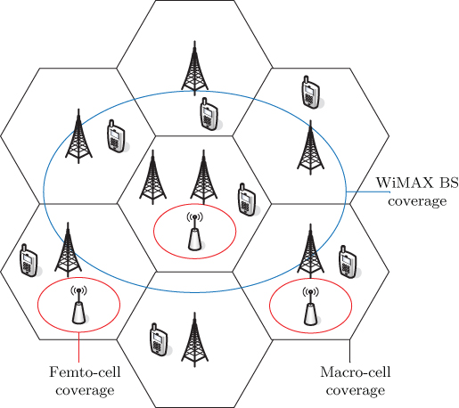
Figure 4.1 Network coverage areas [137]
Let ![]() denote the set of network
denote the set of network ![]() active subscribers in the coverage area of BS
active subscribers in the coverage area of BS ![]() . The set of active MTs in the geographical region is denoted by
. The set of active MTs in the geographical region is denoted by ![]() . MTs are equipped with multiple radio interfaces and multi-homing capabilities. Let
. MTs are equipped with multiple radio interfaces and multi-homing capabilities. Let ![]() and
and ![]() denote the power and bandwidth allocated from network
denote the power and bandwidth allocated from network ![]() BS
BS ![]() to MT
to MT ![]() , respectively.1 In a non-cooperative (single-network) scenario, each MT
, respectively.1 In a non-cooperative (single-network) scenario, each MT ![]() obtains the required radio resources to satisfy a target minimum data rate
obtains the required radio resources to satisfy a target minimum data rate ![]() from its home network. In a cooperative networking scenario, an MT obtains the required radio resources from all networks available at its location. In this section, we do not include a priority mechanism in the problem formulation to differentiate network subscribers and other users when cooperative networking is employed. Hence, all MTs are treated equally by all operators in the cooperative case. Also, it is assumed that the number of radio interfaces for each MT is the same as the number of available BSs/APs at its location.
from its home network. In a cooperative networking scenario, an MT obtains the required radio resources from all networks available at its location. In this section, we do not include a priority mechanism in the problem formulation to differentiate network subscribers and other users when cooperative networking is employed. Hence, all MTs are treated equally by all operators in the cooperative case. Also, it is assumed that the number of radio interfaces for each MT is the same as the number of available BSs/APs at its location.
The channel power gain between network ![]() BS
BS ![]() and MT
and MT ![]() is denoted by
is denoted by ![]() , and it captures both the path loss and fast fading. The path loss is given by
, and it captures both the path loss and fast fading. The path loss is given by ![]() , which is proportional to the distance between network
, which is proportional to the distance between network ![]() BS
BS ![]() and MT
and MT ![]() and
and ![]() denotes the path-loss exponent. The one-sided noise power spectral density is denoted by
denotes the path-loss exponent. The one-sided noise power spectral density is denoted by ![]() .
.
4.2.1 Non-cooperative Single-Network Solution
In this case, different networks do not cooperate with each other for power saving. Hence, each network ![]() BS
BS ![]() allocates its radio resources only to its subscribers, that is, for
allocates its radio resources only to its subscribers, that is, for ![]() , as shown in Figure 4.2a. The objective is to minimize the power consumption of network
, as shown in Figure 4.2a. The objective is to minimize the power consumption of network ![]() while satisfying the required minimum QoS for the network subscribers and the BSs' radio resource constraints. This can be expressed by
while satisfying the required minimum QoS for the network subscribers and the BSs' radio resource constraints. This can be expressed by

where NCS denotes the non-cooperative solution. The total power consumption for network ![]() ,
, ![]() , is expressed as the summation of the power consumption of the BSs of this network, that is,
, is expressed as the summation of the power consumption of the BSs of this network, that is, ![]() , and
, and ![]() consists of two components, namely the load-independent and load-dependent components, that is,
consists of two components, namely the load-independent and load-dependent components, that is,
The achieved data rate for MT ![]() on the downlink of BS
on the downlink of BS ![]() of home network
of home network ![]() is given by Shannon formula
is given by Shannon formula

The total bandwidth allocated by network ![]() BS
BS ![]() to its subscribers is given by
to its subscribers is given by ![]() .
.

Figure 4.2 Illustration of non-cooperative single-network and cooperative multi-homing radio resource allocation. (a) Non-cooperative single-network solution; (b) Cooperative multi-homing solution
Since the Hessian matrix of ![]() is negative semi-definite [137],
is negative semi-definite [137], ![]() is concave in
is concave in ![]() and
and ![]() . As a result, (4.1) minimizes a linear objective function over a convex set (as the first constraint in (4.1) is convex in
. As a result, (4.1) minimizes a linear objective function over a convex set (as the first constraint in (4.1) is convex in ![]() and
and ![]() and the second and third constraints are linear in
and the second and third constraints are linear in ![]() and
and ![]() ). Thus, (4.1) is a convex optimization problem [142].
). Thus, (4.1) is a convex optimization problem [142].
Since (4.1) is a convex optimization problem, it can be solved efficiently by each network BS in polynomial time complexity to find a green downlink radio resource allocation (i.e. ![]() and
and ![]() ) for the network subscribers.
) for the network subscribers.
4.2.2 Win–Win Cooperative Solution
In a heterogeneous networking environment, networks can cooperate in radio resource allocation to achieve power saving, as shown Figure 4.2b. Using the multi-homing capability, MTs aggregate the offered radio resources (i.e. bandwidth and power) from the BSs of different networks with overlapped coverage to satisfy the required minimum QoS and the bandwidth and power constraints of different BSs, to yield power saving for service providers. However, in a multi-operator system, where BSs with overlapped coverage are operated by different service providers, a rationale service provider prefers to work independently (similar to the previous subsection) if its power consumption through cooperation is higher than the NCS. Consequently, in order to promote cooperation for power saving among service providers, Nash bargain games [143] can be used to offer a cooperation incentive radio resource allocation that guarantees mutual benefit (power saving) among different service providers. In this case, the players of the game are the service providers, which are given by the set ![]() . Define
. Define ![]() as the set of game strategies of the
as the set of game strategies of the ![]() networks, that is, (
networks, that is, (![]() ,
, ![]()
![]() , where NBS denotes the Nash bargain solution and
, where NBS denotes the Nash bargain solution and ![]() if
if ![]() is not in the coverage area of network
is not in the coverage area of network ![]() BS
BS ![]() . Let
. Let ![]() be the space of the radio resource allocation strategies, expressed by
be the space of the radio resource allocation strategies, expressed by

where ![]() is obtained by replacing NCS by NBS in (4.3),
is obtained by replacing NCS by NBS in (4.3), ![]() , and
, and
Assuming (4.1) is feasible, the constraint set (4.1) forms a sub-space of ![]() . This can be easily shown by observing that the constraints in (4.1) can be written as the constraints in (4.4) with
. This can be easily shown by observing that the constraints in (4.1) can be written as the constraints in (4.4) with ![]()
![]() . Hence, the constraint set (4.1) is a special case of
. Hence, the constraint set (4.1) is a special case of ![]() .
.
We aim to find a feasible sub-space ![]() with radio resource allocation that results in total power consumption
with radio resource allocation that results in total power consumption ![]() less than or equal to
less than or equal to ![]()
![]() . In Nash bargain game theory,
. In Nash bargain game theory, ![]() is referred to as the initial agreement point. Define
is referred to as the initial agreement point. Define ![]() as a set of network power consumptions satisfying the initial agreement point for
as a set of network power consumptions satisfying the initial agreement point for ![]() . A mapping
. A mapping ![]() is a symmetric NBS if it satisfies the following axioms [143]:
is a symmetric NBS if it satisfies the following axioms [143]:
- 1.
 is Pareto optimal, that is, there exists no other radio resource allocation that results in a superior performance for all networks simultaneously.
 - 2.
 is independent of irrelevant alternatives, that is, if the feasible set shrinks but the radio resource allocation remains feasible, the radio resource allocation for the smaller feasible set will be the same.
 - 3.
 is invariant with respect to affine transformations, that is, if
  is the solution of
  and
and  is a positive linear transformation,
  is the solution of
  .
. - 4.
 provides symmetry, that is, networks with same power consumption in the non-cooperative solution achieve same power saving in the cooperative case.
An asymmetric NBS [144] enables different networks to have different bargain powers in the game, which eventually affects the power saving outcomes for each network. Such a model is very useful to represent the resource availability at different operators (i.e. their capabilities). For instance, one operator may have high network capacity and hence should be able to have more influence on the game outcome.
Let ![]() be the non-empty subset of networks that can achieve strictly superior performance through cooperation. There exist a bargaining solution and unique bargain point for the win–win cooperative downlink green radio resource allocation problem, which is obtained by solving
be the non-empty subset of networks that can achieve strictly superior performance through cooperation. There exist a bargaining solution and unique bargain point for the win–win cooperative downlink green radio resource allocation problem, which is obtained by solving

where ![]() denotes the bargain power of network
denotes the bargain power of network ![]() .
.
In order to prove the existence of a unique bargain point for the win–win cooperative solution, we first prove that ![]() is compact and convex. From (4.4),
is compact and convex. From (4.4), ![]() is closed and bounded, and hence it is compact. As
is closed and bounded, and hence it is compact. As ![]() is concave in
is concave in ![]() and
and ![]() ,
, ![]() is a sum of concave functions in
is a sum of concave functions in ![]() and
and ![]() . Hence, the first constraint in (4.4) is convex. As
. Hence, the first constraint in (4.4) is convex. As ![]() is described by convex and linear constraints, it is convex. From Theorem 2.1 in [145], since
is described by convex and linear constraints, it is convex. From Theorem 2.1 in [145], since ![]()
![]() are linear functions defined on the convex and compact set
are linear functions defined on the convex and compact set ![]() , the cooperative downlink green radio resource allocation has a unique bargain point, which is obtained by solving (4.6).
, the cooperative downlink green radio resource allocation has a unique bargain point, which is obtained by solving (4.6).
The optimization problem (4.6) is solved for ![]() . Networks
. Networks ![]() follow the NCS. One way to reflect the bargain power
follow the NCS. One way to reflect the bargain power ![]() of network
of network ![]() in (4.6) is based on the ratio of the total bandwidth available at network
in (4.6) is based on the ratio of the total bandwidth available at network ![]() to the total bandwidth available in all networks in
to the total bandwidth available in all networks in ![]() , that is,
, that is,

From Theorem 2.2 in [145], as ![]() is injective over the constraint set in (4.6)
is injective over the constraint set in (4.6) ![]() , an equivalent form to (4.6) is given by
, an equivalent form to (4.6) is given by

From (4.8), it is evident that the asymmetric Nash bargain game (4.6) promotes weighted proportional fairness in power saving among the networks [144]. With equal bargain powers (i.e. symmetric Nash bargain game), proportional fairness is guaranteed among different networks.
As ![]() is concave and positive, for
is concave and positive, for ![]() ,
, ![]() is also concave [142]. Hence, the objective function of (4.8) is concave, since it is expressed as the sum of concave functions. In addition, the constraint set of (4.8) is convex. Consequently, (4.8) maximizes a concave function over a convex set, and therefore, it represents a convex optimization program.
is also concave [142]. Hence, the objective function of (4.8) is concave, since it is expressed as the sum of concave functions. In addition, the constraint set of (4.8) is convex. Consequently, (4.8) maximizes a concave function over a convex set, and therefore, it represents a convex optimization program.
The Lagrangian function for (4.8) is given by
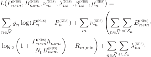

where ![]() ,
, ![]() ,
, ![]() and
and ![]() are the Lagrangian multipliers for the data rate constraint of MT
are the Lagrangian multipliers for the data rate constraint of MT ![]() , maximum bandwidth and power constraints for network
, maximum bandwidth and power constraints for network ![]() BS
BS ![]() , and power saving constraint for network
, and power saving constraint for network ![]() , respectively. As (4.8) is a convex optimization problem, strong duality exists and we can solve (4.8) through its dual problem [142]. The dual function is expressed as
, respectively. As (4.8) is a convex optimization problem, strong duality exists and we can solve (4.8) through its dual problem [142]. The dual function is expressed as

Thus, the dual problem is formulated as
We solve (4.10) and (4.11) to find the optimal joint bandwidth and power allocation for cooperative green communications.
4.2.2.1 Downlink Power Allocation at Each Network
In the following, we derive the optimal allocated power at each network BS, given the bandwidth allocation ![]() and Lagrangian multipliers
and Lagrangian multipliers ![]() and
and ![]() . Applying the Karush–Kuhn–Tucker (KKT) conditions [142], it follows that
. Applying the Karush–Kuhn–Tucker (KKT) conditions [142], it follows that
It turns out that

where ![]() is a projection on the positive quadrant to account for
is a projection on the positive quadrant to account for ![]() and
and ![]() is given by the solution of (4.1).
is given by the solution of (4.1).
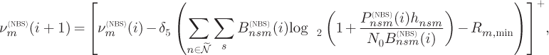
The optimal dual variable ![]() guarantees that the total allocated power by each BS satisfies its maximum power constraint and can be found using the gradient descent method as follows
guarantees that the total allocated power by each BS satisfies its maximum power constraint and can be found using the gradient descent method as follows

where ![]() is an iteration index and
is an iteration index and ![]() is a small step size.
is a small step size.
Similarly, the optimal dual variable ![]() guarantees that the total power allocation by network
guarantees that the total power allocation by network ![]() , using the cooperative approach, is smaller than that obtained via the non-cooperative approach. Applying the gradient descent method, we have
, using the cooperative approach, is smaller than that obtained via the non-cooperative approach. Applying the gradient descent method, we have
where ![]() is a sufficiently small step size.
is a sufficiently small step size.
It can be observed from (4.13) that the power allocation ![]() is a function of the total power consumption
is a function of the total power consumption ![]() , which is also a function of
, which is also a function of ![]() . As a result,
. As a result, ![]() is obtained by updating
is obtained by updating ![]() in an iterative way as follows [146]
in an iterative way as follows [146]

where ![]() is an iteration index and
is an iteration index and ![]() is a sufficiently small step size. Algorithm 4.2.1 describes the optimal power allocation at each network, and
is a sufficiently small step size. Algorithm 4.2.1 describes the optimal power allocation at each network, and ![]() and
and ![]() denote the number of iterations required for convergence.
denote the number of iterations required for convergence.

4.2.2.2 Downlink Bandwidth Allocation at Each Network 
In the following, we derive the optimal allocated bandwidth at each network BS, given the calculated power allocation ![]() and Lagrangian multiplier
and Lagrangian multiplier ![]() . Applying the KKT conditions, we have
. Applying the KKT conditions, we have
Therefore, it follows that

The allocated bandwidth ![]() can be found as the positive real root of (4.18) using Newton's method.
can be found as the positive real root of (4.18) using Newton's method.
The optimal dual variable ![]() guarantees that the total allocated bandwidth by each BS satisfies its maximum bandwidth constraint and can be found using the gradient descent method as follows
guarantees that the total allocated bandwidth by each BS satisfies its maximum bandwidth constraint and can be found using the gradient descent method as follows

where ![]() is a sufficiently small step size.
is a sufficiently small step size.
Algorithm 4.2.2 describes the optimal bandwidth allocation at each network.

4.2.2.3 Downlink Joint Optimal Bandwidth and Power Allocation
The Lagrangian multiplier ![]() is used by each MT
is used by each MT ![]() to coordinate the radio resources allocated by different networks such that the MT minimum required data rate is satisfied. The Lagrangian multiplier
to coordinate the radio resources allocated by different networks such that the MT minimum required data rate is satisfied. The Lagrangian multiplier ![]() can be found using a gradient descent method as follows
can be found using a gradient descent method as follows
where ![]() is a sufficiently small step size.
is a sufficiently small step size.
Algorithm 4.2.3 describes the optimal joint bandwidth and power allocation that satisfies the MTs' required QoS and exhibit win–win power saving for the service providers.

To summarize, network operators should first solve (4.1) to find the NCS (the initial agreement point). Since (4.1) is a convex optimization problem, it can be solved efficiently by each network BS in polynomial time complexity. Then, networks that belong to ![]() solve (4.8) to find the NBS. The set of networks belonging to
solve (4.8) to find the NBS. The set of networks belonging to ![]() is the one that makes (4.8) feasible. Determining
is the one that makes (4.8) feasible. Determining ![]() presents an upper bound complexity on the order of
presents an upper bound complexity on the order of ![]() . Such a complexity is not high since the number of operators within a region,
. Such a complexity is not high since the number of operators within a region, ![]() , is expected to be in the range
, is expected to be in the range ![]() . The complexity of obtaining the NBS using the Algorithm 4.2.3 reduces to solving the dual problem, which presents a complexity upper bounded by
. The complexity of obtaining the NBS using the Algorithm 4.2.3 reduces to solving the dual problem, which presents a complexity upper bounded by ![]() , where
, where ![]() and
and ![]() are the numbers of MTs in
are the numbers of MTs in ![]() and networks in
and networks in ![]() . Hence, it has a linear complexity in the number of MTs
. Hence, it has a linear complexity in the number of MTs ![]() , network operators
, network operators ![]() and BSs
and BSs ![]() . Algorithms 4.2.1–4.2.3 are guaranteed to converge to an optimal solution using sufficiently small step sizes, since (4.8) is convex.
. Algorithms 4.2.1–4.2.3 are guaranteed to converge to an optimal solution using sufficiently small step sizes, since (4.8) is convex.
4.2.3 Benchmark: Sum Minimization Solution
In this subsection, we present a benchmark for power-efficient cooperative radio resource allocation in a heterogeneous wireless medium. The benchmark is referred to as a sum minimization solution as it uses cooperation among networks to minimize the total (sum) power consumption in the geographical region. Hence, MTs are allocated radio resources (i.e. bandwidth and power) from the BSs of different networks and aggregate them using the multi-homing capability to satisfy its required QoS while minimizing the networks' total power consumption and satisfying the radio resource constraints. This can be expressed by

where SMS denotes the sum minimization solution. Similar to (4.8), (4.21) is a convex optimization problem as it involves the minimization of a linear function over a convex constraint set. Hence, (4.21) can be solved efficiently in polynomial time complexity to find a green downlink multi-homing resource allocation (i.e. ![]() and
and ![]() ).
).
4.2.4 Performance Evaluation
This section evaluates the performance of the win–win cooperative green radio resource allocation mechanism based on the NBS, which is described by the Algorithms 4.2.1–4.2.3, and it is compared with two benchmarks. The first benchmark is the SMS that is given by the radio resource allocation in (4.21), which resembles the radio resource allocation schemes in [32, 33] and [36]. The second benchmark is the NCS that is given by the radio resource allocation in (4.1), which resembles the radioresource allocation strategies in [17, 38, 79, 111, 147–150] and [151]. Simulations are performed for a geographical region that is covered by two BSs belonging to two different networks. The angle between the horizontal axis and the line joining the two BSs is randomly chosen following a uniform distribution in ![]() . Each BS has a maximum power constraint of 191 W, static power consumption of 77 W, and drain efficiency of
. Each BS has a maximum power constraint of 191 W, static power consumption of 77 W, and drain efficiency of ![]() for the power amplifier, that is,
for the power amplifier, that is, ![]() [152]. MTs are uniformly distributed in the geographical region with 50 and 30 MTs as the subscribers of the first and second network, respectively. All MTs require the same minimum data rate 0.1 Mbps. Furthermore, MTs are subject to independent Rayleigh fading channels and path-loss exponent
[152]. MTs are uniformly distributed in the geographical region with 50 and 30 MTs as the subscribers of the first and second network, respectively. All MTs require the same minimum data rate 0.1 Mbps. Furthermore, MTs are subject to independent Rayleigh fading channels and path-loss exponent ![]() with both BSs. The one-sided noise power spectral density is
with both BSs. The one-sided noise power spectral density is ![]() dBm/Hz.
dBm/Hz.
We present three sets of results. In the first set, which is depicted in Figures 4.3 and 4.4, it is assumed that all the subscribers of the first network enjoy good channel conditions with both BSs, while the number of second network subscribers who enjoy good channel conditions with the first network BS is varied. As a result, all network 1 subscribers can connect to both BSs, while only a fraction ![]() of network 2 subscribers can connect to the BS of the first network. The rest of the second network subscribers who cannot connect to the first network BS receive their required radio resources only from their home network, that is, network 2. In this set of results, the BSs are separated by 250 m. Also, the total bandwidth available at each BS is 10 MHz. Hence, both networks have equal bargain power
of network 2 subscribers can connect to the BS of the first network. The rest of the second network subscribers who cannot connect to the first network BS receive their required radio resources only from their home network, that is, network 2. In this set of results, the BSs are separated by 250 m. Also, the total bandwidth available at each BS is 10 MHz. Hence, both networks have equal bargain power ![]() for
for ![]() . The second set of results, which is given by Figures 4.5 and 4.6, investigates the system performance for different bargain powers of the networks. In particular, we vary the total bandwidth available for network 2 in the range
. The second set of results, which is given by Figures 4.5 and 4.6, investigates the system performance for different bargain powers of the networks. In particular, we vary the total bandwidth available for network 2 in the range ![]() MHz and fix the total bandwidth available for network 1 to 10 MHz. As a result, the bargain power of network 2 varies in the range
MHz and fix the total bandwidth available for network 1 to 10 MHz. As a result, the bargain power of network 2 varies in the range ![]() and
and ![]() . In this set of results, all MTs are able to connect to both networks using their multi-homing capabilities. Again, the distance between both BSs is 250 m. The last set of results, which is depicted in Figures 4.7 and 4.8, assumes a variable distance between the two BSs. Hence, we fix the position of the second BS and move the first BS away from it within a distance range of
. In this set of results, all MTs are able to connect to both networks using their multi-homing capabilities. Again, the distance between both BSs is 250 m. The last set of results, which is depicted in Figures 4.7 and 4.8, assumes a variable distance between the two BSs. Hence, we fix the position of the second BS and move the first BS away from it within a distance range of ![]() m. The total bandwidth available at each BS is 10 MHz and all MTs are able to connect to both networks using their multi-homing capabilities. The three sets of results represent situations where cooperation is not always beneficial for network 2. Simulation results present the confidence interval for a
m. The total bandwidth available at each BS is 10 MHz and all MTs are able to connect to both networks using their multi-homing capabilities. The three sets of results represent situations where cooperation is not always beneficial for network 2. Simulation results present the confidence interval for a ![]() confidence level.
confidence level.
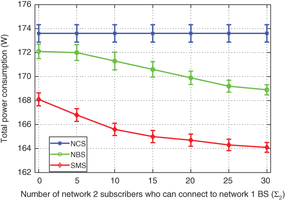
Figure 4.3 Total power consumption in the geographical region with different  [137]. The BSs are separated by 250 m. The total bandwidth available at each BS is 10 MHz

Figure 4.4 Power consumption for each BS with different  [137]. The BSs are separated by 250 m. The total bandwidth available at each BS is 10 MHz

Figure 4.5 Total power consumption in the geographical region with different  [137]. The distance between both BSs is 250 m. The total bandwidth available at BS 1 is 10 MHz and BS 2 is in the range
  MHz
MHz

Figure 4.6 Power consumption for each BS with different  [137]. The distance between both BSs is 250 m. The total bandwidth available at BS 1 is 10 MHz and BS 2 is in the range
  MHz
MHz

Figure 4.7 Total power consumption in the geographical region with different separation distances between the two BSs [137]. The total bandwidth available at each BS is 10 MHz

Figure 4.8 Power consumption for each BS with different separation distances between the two BSs [137]. The total bandwidth available at each BS is 10 MHz
Figure 4.3 shows a plot of total power consumption in the geographical region, ![]() against the number of network 2 subscribers who can connect to the BSs of both networks,
against the number of network 2 subscribers who can connect to the BSs of both networks, ![]() . The NCS total power consumption is independent of
. The NCS total power consumption is independent of ![]() as in the NCS each network allocates its radio resources only to its own subscribers, regardless of the fraction of users who are able to connect to both networks using multi-homing. For the cooperative solutions (SMS and NBS), the total power consumption in the geographical region is reduced as more subscribers from network 2 are able to connect to both BSs. This is because, with
as in the NCS each network allocates its radio resources only to its own subscribers, regardless of the fraction of users who are able to connect to both networks using multi-homing. For the cooperative solutions (SMS and NBS), the total power consumption in the geographical region is reduced as more subscribers from network 2 are able to connect to both BSs. This is because, with ![]() , more opportunities are created by the cooperative solutions through multi-homing to satisfy the users' required QoS at reduced network power consumption. While both cooperative solutions achieve lower power consumption compared to the NCS, only the NBS offers cooperation incentives for power minimization in comparison with the SMS, as will be shown next.
, more opportunities are created by the cooperative solutions through multi-homing to satisfy the users' required QoS at reduced network power consumption. While both cooperative solutions achieve lower power consumption compared to the NCS, only the NBS offers cooperation incentives for power minimization in comparison with the SMS, as will be shown next.
Figure 4.4 shows a plot of the total power consumption for each network BS, ![]() against
against ![]() . For the entire range of
. For the entire range of ![]() , the SMS reduces the power consumption for network 1 BS (SMS1
, the SMS reduces the power consumption for network 1 BS (SMS1 ![]() NCS1) significantly at the cost of an increase in the power consumption of network 2 BS (SMS2
NCS1) significantly at the cost of an increase in the power consumption of network 2 BS (SMS2 ![]() NCS2). For
NCS2). For ![]() , SMS1 is decreasing with
, SMS1 is decreasing with ![]() , since more power saving opportunities can be achieved with
, since more power saving opportunities can be achieved with ![]() within this range. For
within this range. For ![]() , SMS1 slightly increases with
, SMS1 slightly increases with ![]() , as more users from network 1 now can receive part of their required resources from network 1; however, still SMS1 is significantly less than NCS1, yet SMS2
, as more users from network 1 now can receive part of their required resources from network 1; however, still SMS1 is significantly less than NCS1, yet SMS2 ![]() NCS2. Consequently, within
NCS2. Consequently, within ![]() , the SMS does not offer an incentive for network 2 BS to cooperate with network 1 BS for power minimization. On the contrary , the NBS always results in a power consumption for both BSs (NBS1 for BS1 and NBS2 for BS2) that is less than or equal to the NCS. Consequently, the NBS always guarantees mutual benefit of power saving for both networks. Hence, within the win–win cooperative framework, both networks have incentives to cooperate for power saving.
, the SMS does not offer an incentive for network 2 BS to cooperate with network 1 BS for power minimization. On the contrary , the NBS always results in a power consumption for both BSs (NBS1 for BS1 and NBS2 for BS2) that is less than or equal to the NCS. Consequently, the NBS always guarantees mutual benefit of power saving for both networks. Hence, within the win–win cooperative framework, both networks have incentives to cooperate for power saving.
Figure 4.5 shows the total power consumption in the geographical region for different bargain powers of the networks. Both the NCS and SMS are independent of the bargain power of the network. For the NBS, as the bargain power of network 2 increases, less power saving is achieved in the geographical region. The rationale behind such a behaviour is explained using the next result.
Figure 4.6 shows the total power consumption for each network BS versus ![]() . The NBS represents a weighted proportional fair solution. For a larger value of
. The NBS represents a weighted proportional fair solution. For a larger value of ![]() , more emphasis is given to power saving for the second network BS. This is met by lowering the importance of power saving at the first network BS. While such a behaviour limits the power saving opportunities, which is clear in Figure 4.5 for the NBS compared with the SMS, it gives a flexibility to the cooperating entities to achieve a better bargain (power saving) based on their capabilities (e.g. total available bandwidth). This is clear from the behaviour of NBS1 and NBS2 compared with NCS1 and NCS2, respectively, for different bargain power values. On the contrary, for the SMS, regardless of the capabilities of network 2 (total available bandwidth as compared with network 1), it always achieves a higher power consumption than the NCS (as given by SMS2 compared with NCS2), which does not motivate the second network to cooperate, unlike the NBS (as given by NBS2 compared with NCS2).
, more emphasis is given to power saving for the second network BS. This is met by lowering the importance of power saving at the first network BS. While such a behaviour limits the power saving opportunities, which is clear in Figure 4.5 for the NBS compared with the SMS, it gives a flexibility to the cooperating entities to achieve a better bargain (power saving) based on their capabilities (e.g. total available bandwidth). This is clear from the behaviour of NBS1 and NBS2 compared with NCS1 and NCS2, respectively, for different bargain power values. On the contrary, for the SMS, regardless of the capabilities of network 2 (total available bandwidth as compared with network 1), it always achieves a higher power consumption than the NCS (as given by SMS2 compared with NCS2), which does not motivate the second network to cooperate, unlike the NBS (as given by NBS2 compared with NCS2).
Figure 4.7 shows the total power consumption in the geographical region for different separation distances among the two BSs. As the first network BS moves further away from the second network BS, the total power consumption increases for both the NCS and NBS, while it first decreases for the SMS and then saturates. Such a behaviour is explained using the following result.
Figure 4.8 shows a plot of the total power consumption for each network BS against the separation distance between the two BSs. For the NCS, as the first BS moves further away from the second BS, the distance between some subscribers of the first network and their home network (network 1 BS) increases, leading to an increased transmission power for BS 1 (and hence an increased total power consumption for BS 1, i.e. NCS1). On the contrary, the transmission power for BS 2 is not much affected due to the fixed location of BS 2. Consequently, the total power consumption in the region increases with the separation distance (as shown in Figure 4.7 for the NCS). For the SMS, as the separation distance increases, the first network BS relies more on the second network BS to serve its faraway subscribers that are in closer proximity to BS 2. Consequently, this increases the transmission power of BS 2 (and hence increases BS 2 total power consumption, i.e. SMS2), while it decreases the transmission power of BS 1 (and hence decreases BS 1 total power consumption, i.e. SMS1). Overall, this decreases the power consumption in the region with the separation distance (as shown in Figure 4.7 for the SMS). While the SMS reduces power consumption of BS 1 (SMS1 ![]() NCS1), it increases the power consumption of BS2 (SMS2
NCS1), it increases the power consumption of BS2 (SMS2 ![]() NCS2). Finally, the NBS always guarantees that the power consumption of both BSs is lower than that of the NCS. In order to keep the second network BS power consumption lower than that corresponding to the NCS (NBS2
NCS2). Finally, the NBS always guarantees that the power consumption of both BSs is lower than that of the NCS. In order to keep the second network BS power consumption lower than that corresponding to the NCS (NBS2 ![]() NCS2), the first network BS has to increase its transmission power to cope up with the increased distance between BS 1 and some MTs; however, BS 1 still achieves lower power consumption than the NCS (NBS1
NCS2), the first network BS has to increase its transmission power to cope up with the increased distance between BS 1 and some MTs; however, BS 1 still achieves lower power consumption than the NCS (NBS1 ![]() NCS1). Hence, this increases the power consumption in the region with the separation distance (as shown in Figure 4.7 for the NBS).
NCS1). Hence, this increases the power consumption in the region with the separation distance (as shown in Figure 4.7 for the NBS).
4.3 IDC Interference-Aware Green Resource Allocation
In this section, we present a minimum power consumption radio resource allocation algorithm for LTE/WiFi networks that takes into account the mutual IDC interference between LTE and WiFi. Such a resource allocation algorithm fits the scenario, where different radio interfaces of the MT run different applications, and hence, the uplink transmission of one radio interface causes interference on the downlink reception of another radio interface that operates in a close frequency band. This is different from the scenario described in the previous section, where all radio interfaces of a given MT serve the downlink reception of one application, and hence, no IDC interference exists.
Consider a network consisting of a WLAN AP overlaid in the coverage of a single-cell LTE BS, whereby ![]() MTs with LTE and WLAN radio interfaces are distributed in the region of interest. Under the typical scenario, where users run different applications on LTE and WLAN interfaces, we consider a scenario where LTE and WLAN operate in adjacent bands in a TDD mode. Therefore, mutual IDC interference exists between the LTEand WLAN interfaces of each user. The LTE BS has a total bandwidth of
MTs with LTE and WLAN radio interfaces are distributed in the region of interest. Under the typical scenario, where users run different applications on LTE and WLAN interfaces, we consider a scenario where LTE and WLAN operate in adjacent bands in a TDD mode. Therefore, mutual IDC interference exists between the LTEand WLAN interfaces of each user. The LTE BS has a total bandwidth of ![]() MHz and a set of channels
MHz and a set of channels ![]() . The total bandwidth is equally divided among the
. The total bandwidth is equally divided among the ![]() channels, each having
channels, each having ![]() channel bandwidth. The channel is assigned to a single user at a given time. However, a user can be assigned to more than one channel. We denote
channel bandwidth. The channel is assigned to a single user at a given time. However, a user can be assigned to more than one channel. We denote ![]() as the channel assignment variable for user
as the channel assignment variable for user ![]() in channel
in channel ![]() , where
, where ![]() if channel
if channel ![]() is assigned to user
is assigned to user ![]() , otherwise,
, otherwise, ![]() . Variables
. Variables ![]() and
and ![]() denote the allocated downlink power and channel gain for user
denote the allocated downlink power and channel gain for user ![]() on channel
on channel ![]() , respectively. Let
, respectively. Let ![]() and
and ![]() denote the noise power spectral density and IDC interference on LTE channel
denote the noise power spectral density and IDC interference on LTE channel ![]() assigned to user
assigned to user ![]() , respectively. Using Shannon formula, the maximum achievable data rate for user
, respectively. Using Shannon formula, the maximum achievable data rate for user ![]() in the LTE network downlink can be expressed by
in the LTE network downlink can be expressed by

For the WLAN, each AP is assigned a single channel and users share this channel in a TDMA manner. This can be achieved by an enhanced version of the DCF [130]. The user is assigned the whole AP bandwidth (![]() ) in its allocated time fraction denoted by
) in its allocated time fraction denoted by ![]() . Hence, the WLAN downlink data rate of user
. Hence, the WLAN downlink data rate of user ![]() is expressed as
is expressed as

where ![]() and
and ![]() denote the allocated downlink power and channel gain for MT
denote the allocated downlink power and channel gain for MT ![]() , respectively,
, respectively, ![]() is the noise power at the WLAN receiver, and
is the noise power at the WLAN receiver, and ![]() represents the LTE interference on the WLAN signal.
represents the LTE interference on the WLAN signal.
The IDC interference that affects LTE channel ![]() when it is allocated to user
when it is allocated to user ![]() ,
, ![]() , and the IDC interference at the WLAN receiver,
, and the IDC interference at the WLAN receiver, ![]() , are given in (3.2) and (3.4), respectively, as function of the interfering WLAN uplink power allocated by MT
, are given in (3.2) and (3.4), respectively, as function of the interfering WLAN uplink power allocated by MT ![]() ,
, ![]() , the interfering LTE uplink power allocated by MT
, the interfering LTE uplink power allocated by MT ![]() on channel
on channel ![]() ,
, ![]() and the losses due to the antenna isolation at user
and the losses due to the antenna isolation at user ![]() ,
, ![]() .
.
4.3.1 IDC Interference-Aware Resource Allocation Design
The WLAN and LTE uplink transmission powers leak into the downlink reception paths of LTE and WLAN, respectively, as depicted in Figure 3.4. In this subsection,we design a resource allocation mechanism that meets the data rate requirements in the victim downlink path by using a joint channel, time and downlink power radio resource allocation (![]() ,
, ![]() ,
, ![]() and
and ![]() ). The IDC resource allocation problem is formulated with the target of minimizing the downlink transmission power as follows
). The IDC resource allocation problem is formulated with the target of minimizing the downlink transmission power as follows

where ![]() and
and ![]() are the minimum data rate requirements for the LTE and WLAN radios, respectively. The third constraint in (4.25) ensures that each LTE channel is assigned to a single user. The last constraint in (4.25) guarantees that one WLAN user can access the channel at a given time.
are the minimum data rate requirements for the LTE and WLAN radios, respectively. The third constraint in (4.25) ensures that each LTE channel is assigned to a single user. The last constraint in (4.25) guarantees that one WLAN user can access the channel at a given time.
The terms ![]() and
and ![]() in the data rate expressions (4.23) and (4.24) couple the resource allocation of both radios, since the amount of interference depends on the frequency gap between the LTE and WLAN channels allocated to the user. Under the fact that each transceiver for each network can calculate the interference power in its band using (3.2) and (3.4), (4.25) can be solved by letting each BS/AP perform its resource allocation while considering the IDC observed from the other network.
in the data rate expressions (4.23) and (4.24) couple the resource allocation of both radios, since the amount of interference depends on the frequency gap between the LTE and WLAN channels allocated to the user. Under the fact that each transceiver for each network can calculate the interference power in its band using (3.2) and (3.4), (4.25) can be solved by letting each BS/AP perform its resource allocation while considering the IDC observed from the other network.
4.3.1.1 LTE Radio Resource Allocation
Optimizing only for the LTE resources, the decoupled problem has the target of minimizing the LTE transmission power and is constrained by meeting the LTE data rate requirements of all users while considering the IDC interference as follows

Problem (4.25) is an MINLP due to the existence of the binary optimization variable ![]() and the continuous optimization variable
and the continuous optimization variable ![]() . By relaxing the binary constraint
. By relaxing the binary constraint ![]() to take continuous values in the range
to take continuous values in the range ![]() , the optimum power and channel allocation variables can be expressed as follows [153]
, the optimum power and channel allocation variables can be expressed as follows [153]

and
where

The optimal values of the Lagrangian multipliers (![]() ) must satisfy the complementary slackness condition expressed as
) must satisfy the complementary slackness condition expressed as ![]() . The resource allocation solution states that the user presenting the minimum value for
. The resource allocation solution states that the user presenting the minimum value for ![]() is assigned channel
is assigned channel ![]() without any time-sharing with other users. This radio resource assignment converges only in low-dense networks, where the number of users is much lower than the number of channels. However, in high-dense networks, where the number of users is comparable to the number of channels, some channels keep oscillating between two or more users and convergence does not occur. In order to overcome this problem, a priority scheme is proposed to settle the competition between users as follows:
without any time-sharing with other users. This radio resource assignment converges only in low-dense networks, where the number of users is much lower than the number of channels. However, in high-dense networks, where the number of users is comparable to the number of channels, some channels keep oscillating between two or more users and convergence does not occur. In order to overcome this problem, a priority scheme is proposed to settle the competition between users as follows:
- Case 1: Only one user is not assigned any channels among the competing users: The contested channel will be assigned to this user with no other assigned channels.
- Case 2: None of the competing users is assigned a channel: The contested channel will be assigned to the user having the worst channel conditions among the competing users.
The intuition behind this scheme is to allow fairness among users. In Case 1, the winning user is the one with no assigned channels. In Case 2, the channel is assigned to the most needy user who will face even worse channel conditions if it is assigned any channel other than the contested channel.
4.3.1.2 WLAN Radio Resource Allocation
Similarly, in allocating only the WLAN resources, our objective is to minimize the WLAN transmission power while meeting the WLAN data rate requirements of all users and considering the IDC interference. This optimization problem is formulated as follows

Problem (4.29) is a convex optimization problem due to the linearity of the objective function and the last constraint together with the concavity of the first constraint. By applying the Lagrangian duality theory, the optimal power and time fraction allocation can be expressed as follows [127]

The optimal values of the Lagrangian multipliers (![]() and
and ![]() ) can be obtained by enforcing the complementary slackness conditions given by
) can be obtained by enforcing the complementary slackness conditions given by ![]() and
and ![]() .
.
4.3.2 Performance Evaluation
Consider the simultaneous operation of LTE and WLAN radio technologies in one mobile. The WLAN operates on a 22-MHz TDD channel, while the LTE operates on a 5-MHz TDD channel. The design of the WLAN spectrum mask is obtained from the IEEE 802.11 standard [131]. The used LTE spectrum mask is similar to a 5-MHz ISM filter, but shifted to create a pass-band for the LTE channels as carried out by the 3GPP [128]. Interference parameters are summarized in Table 3.1.
We consider an LTE BS located at coordinates ![]() . One WLAN AP is located within the coverage of the LTE BS at coordinates
. One WLAN AP is located within the coverage of the LTE BS at coordinates ![]() with radius of 100 m. Users with LTE and WLAN interfaces are randomly distributed within the WLAN AP coverage. A Rayleigh fading channel model is used to describe the wireless channel between each user and the BS/AP. For the LTE, we consider 20 channels, each having 5-MHz channel bandwidth between 2,300 and 2,400 MHz. The maximum allowable downlink power per channel is 33 dBm. The AP operates on IEEE 802.11 channel 3 (centre frequency equal to 2,422 MHz). WLAN users share this channel in the time domain. The maximum allowable WLAN downlink power for each user is 27 dBm. The rest of simulation parameters are depicted in Table 4.1. We compare the IDC interference-aware resource allocation mechanism with a benchmark defined in [153], which overlooks the IDC interference.
with radius of 100 m. Users with LTE and WLAN interfaces are randomly distributed within the WLAN AP coverage. A Rayleigh fading channel model is used to describe the wireless channel between each user and the BS/AP. For the LTE, we consider 20 channels, each having 5-MHz channel bandwidth between 2,300 and 2,400 MHz. The maximum allowable downlink power per channel is 33 dBm. The AP operates on IEEE 802.11 channel 3 (centre frequency equal to 2,422 MHz). WLAN users share this channel in the time domain. The maximum allowable WLAN downlink power for each user is 27 dBm. The rest of simulation parameters are depicted in Table 4.1. We compare the IDC interference-aware resource allocation mechanism with a benchmark defined in [153], which overlooks the IDC interference.
Table 4.1 Simulation parameters [127]
| Parameter | Value |
| LTE path-loss model | |
| WLAN path-loss model | |
| LTE noise figure | 9 dBm |
| LTE noise power density | |
| WLAN noise power | |
| Rate requirement per LTE user ( |
5 Mbps |
| Rate requirement per WLAN user ( |
2 Mbps |
Figure 4.9 depicts the achieved data rate and consumed power in the LTE network. As expected, the IDC interference-aware mechanism outperforms the benchmark in terms of power consumption. However, both mechanisms achieve the same data rate. In the IDC interference-aware mechanism, the users are assigned channels having the least interference effects and fading conditions. In the benchmark, the user selects the channels based on the fading conditions only without taking into consideration that some of these channels may experience high IDC interference. When the user is assigned a highly interfered channel, it keeps increasing its transmission power without achieving the required data rate till it is assigned additional channels based on the water-filling principle. Then, using these additional channels, the user meets the required throughput at the expense of wasting some of its power on the highly interfered channels.

Figure 4.9 LTE network performance [127]. (a) Achieved data rate; (b) power consumption
The IDC interference-aware LTE resource allocation mechanism uses the least interfered LTE channels, which present sufficient frequency separation from the WLAN channel. Therefore, the WLAN radio does not experience high interference and achieves high data rate with low power consumption, as depicted in Figure 4.10. By contrast, the LTE benchmark uses the highly interfered channels, which are closest to the WLAN band. These channels produce high interference to the WLAN channel. Therefore, in the benchmark WLAN resource allocation mechanism, some users consume their maximum transmission power and do not meet the required rate, as depicted in Figure 4.10. The WLAN AP has only one channel to offer to users. When this channel is subjected to high interference, the WLAN performance is severely affected unlike the LTE BS that presents a variety of channels.

Figure 4.10 WLAN performance [127]. (a) Achieved data rate; (b) power consumption
4.4 Summary
This chapter presents two radio resource allocation mechanisms for green downlink communications. The first mechanism supports green communications in a multi-operator heterogeneous wireless medium. It guarantees mutual benefits in power saving among different service providers. The mechanism is based on a Nash bargain game among different service providers and is implemented in a decentralized manner. The Nash bargain strategy guarantees mutual benefits among different service providers as compared with the total (sum) power minimization approach, and hence, it offers incentives for different networks to cooperate. The second mechanism accounts for the filtering characteristics of the transceivers as well as their physical characteristics (e.g. antenna isolation) to alleviate the IDC interference, which can severely limit the performance of both the WLAN and LTE networks. The resource allocation mechanism minimizes not only the consumed power but also the effects of IDC interference implicitly.