
52 Handb ook of Big Data
(m −r) ×n matrix representing the dynamics of noncharacteristic generators; x is an r ×n
matrix and can be calculated from Equation 4.5; and κ
ξ
is an r × r square matrix; κ
¯
ξ
is an (m − r) × r matrix. Normally, κ
ξ
is invertible. We have two different approaches to
finding the approximate linear relations between
¯
ξ and ξ. The first approach is to solve the
following overdetermined equation:
¯
ξ = Cξ (4.8)
where C is an (m − r) × r matrix and can be determined by the least-squares method,
namely, C =
¯
ξ[(ξξ
T
)
−1
ξ]
T
. Another approach is to use the approximate linear relations in
Equation 4.8. According to Equation 4.8, we have
ξ ≈ κ
ξ
x (4.9)
and
¯
ξ ≈ κ
¯
ξ
x (4.10)
Premultiplying κ
−1
ξ
on both sides of Equation 4.9 yields
x ≈ κ
−1
ξ
ξ (4.11)
Substituting Equation 4.11 into 4.10 yields
¯
ξ ≈ κ
¯
ξ
κ
−1
¯
ξ
ξ (4.12)
Equation 4.8 or 4.12 establishes the approximate linear relations between the rotor angle
dynamics of characteristic generators and that of noncharacteristic generators. The dyna-
mics of all generators in the original system then can be reconstructed by using only the
dynamic responses from characteristic generators.
4.2.1.2.4 Generalization to High-Or der Models
In classical models, it is assumed that the magnitude of the generator internal voltage E
is
constant, and only its rotor angle δ changes after a disturbance. In reality, with the generator
excitation system, E
will also respond dynamically to the disturbance. The dynamics of E
can be treated in the same way as the rotor angle δ in the above-mentioned model reduction
method to improve the reduced model, except thatthesetofcharacteristic generators needs
to be determined from δ.Thisway,bothδ and E
of noncharacteristic generators will be
represented in the reduced model using those of the characteristic generators.
4.2.1.2.5 Online Application of the DEAR Method
For offline studies, the DEAR process can be performed at different conditions and operating
points of the target system (external area) to obtain the corresponding reduced models.
For online applications, however, computational cost may be very high if SVD has to be
calculated every time the system configuration changes. A compromise can be made by
maintaining a fixed set of characteristic generators, which is determined by doing SVDs
for multiple scenarios offline and taking the super set of the characteristic generators from
each scenario. During real-time operation of the system, the approximation matrix C from
Equation 4.8 used for feature reconstruction, is updated (e.g., using the recursive least-
squares method) based on a few seconds data right after a disturbance. This way, SVD is
not needed every time after a different disturbance occurs.
4.2.1.3 Case Study
In this section, the IEEE 145-bus, 50-machine system [5] in Figure 4.1 is investigated. There
are 16 and 34 machines in the internal and external areas, respectively. Generator 37 at

Integrate Big Data for Better Operation, Control, and Protection of Power Systems 53
External area
1
2
6
114
113
104
66
8
9
69
11
72
12
13
70
100 103
58
14
15
17
59
21 20 19 18
81
74
25
73
22
83
60
94
97
124
125
121
120
122
107 79
80
130
90
95
123
133
138
118
117
116
115
145
144 143 142
141
140
139
137
136
135
134
132
131
128
127
129
92
78 30 23
106
105
82
108
109
27
75
29
91
24
76
77
96
89
28
31
2616
98
71
112
111
67
57
101
102
49
40
53
56
63
10
32
93
33
99
87 88
45
42
41
48
44
49
46
47
50
51
61 86
85
55
52
54
126
119
62
64
65
68
43
34
35
37
38
39
84
36
110
5
4
3
Internal area
FIGURE 4.1
IEEE 50 machine system. (From S. Wang et al., IEEE Trans. Pattern Anal. Mach. Intell.,
29, 2049–2059, 2014.)
Bus 130 in the internal area is chosen as the reference machine. All generators are mod-
eled using classical models. A three-phase, short-circuit fault (F1) is configured on Lines
116–136 at Bus no. 116 at t = 1 s. The fault lasts for 60 ms, and then the line is tripped to
clear the fault. Postfault rotor angle dynamics in the time interval of 1.2 ≤ t ≤ 5sareana-
lyzed to perform model reduction, using inertial aggregation [6] (one of the coherency-based
reduction methods) and the DEAR method, so that their performance can be compared.
Many methods are available for coherency identification. In this case study, the principal
component analysis method presented by Anaparthi et al. [1] and Moore [12] is chosen
to identify coherency groups, and the MATLAB
clustering toolbox is used to aid the
analysis. Clustering results according to the rotor angle dynamics in the external area are
shown in Figure 4.2. In Figure 4.2, the horizontal axis represents generator numbers, and
the vertical axis scales distances between generator groups. Here the distance is defined in
the three-dimensional Euclidean space expanded by the first three columns of the matrix T
in Equation 4.5. Depending on the distance selected between clusters, different number of
coherency groups can be obtained. For example, at a distance larger than 9, two groups are
formed (level-2 clustering). Generators 23, 30, and 31 comprise one group, and the other gen-
erators comprise another group. Similarly, there are 10 generator groups at level 10, which
are shown in the following: Group 1 (generators 30, 31); Group 2 (generator 23); Group 3
(generators 9 and 10); Group 4 (generator 16); Groups 5 (generators 7, 13, and 15); Group 6
(generator 3); Group 7 (generators 32 and 36); Group 8 (generators 8, 18, 25, 33, 34, and 35);
Group 9 (generators 2 and 6); Group 10 (generators 1, 4, 5, 11, 12, 14, 17, 19–22, 24, 26,
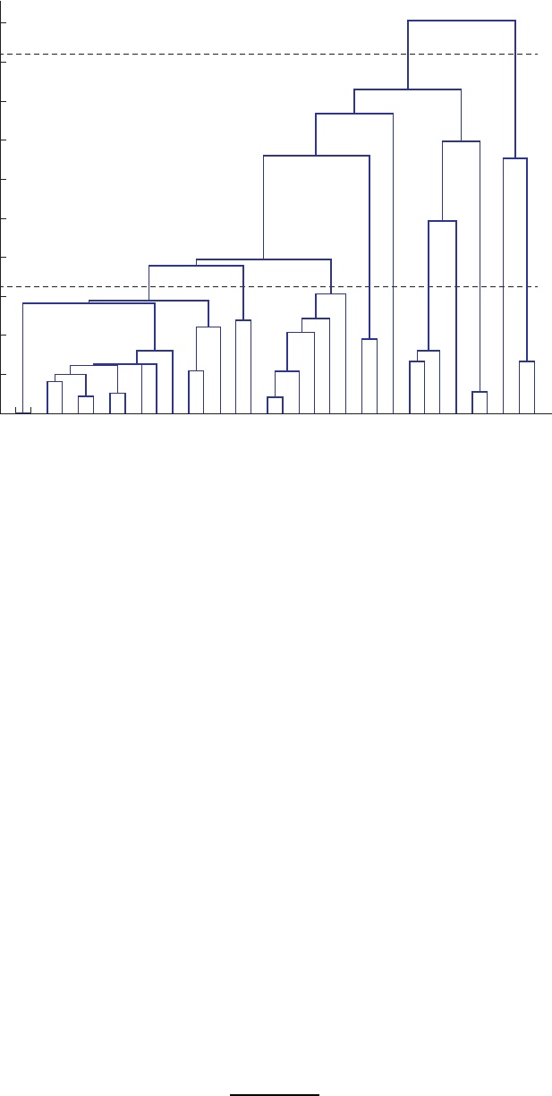
54 Handb ook of Big Data
10
10
Level 2
Level 10
22,27,1,5,17,20,19,21,24,4,12,11,26,14,2,6,8,35,34,18,33,25,32,36,3,7,13,15,16,9,10,23,30,31
Machine number
9
9
8
8
7
7
6
6
5
5
Distance
4
4
3
3
2
2
1
1
2
1
0
FIGURE 4.2
Coherent groups clustering. (From S. Wang et al., IEEE Trans. Pattern Anal. Mach. Intell.,
29, 2049–2059, 2014.)
and 27). Fewer groups result in a simpler system. The normalized (i.e., subtracted by the
mean value of the data and divided by its standard deviation) angle dynamics of the 10
groups at level 10 are shown in Figure 4.3, where coherency can be observed between gen-
erators in the same group. These coherent machines are then aggregated using the inertial
aggregation method reported by Chow et al. [6]. Finally, we obtain a reduced system with
10 aggregated generators for the external system. Following the procedure described above,
the optimal orthogonal bases are first obtained by Equations 4.3 and 4.5 and by setting
r = 10. These 10 basis vectors are shown as the blue solid lines in Figure 4.4. Then, the
corresponding 10 characteristic generators are identified using Equation 4.7. The rotor angle
dynamics of these characteristic generators are shown as dashed red lines in Figure 4.4. An
approximate linear relation between the characteristic generators and the noncharacteristic
generators is then established to get the reduced model. Notice that, in this case, δ
2
has the
highest similarity to orthogonal bases x
7
and x
8
. Therefore, the set of characteristic gen-
erators contains only nine elements, which is ξ =[δ
27
δ
3
δ
15
δ
30
δ
36
δ
23
δ
2
δ
18
δ
4
]
T
. With
the reduced models developed using both coherency aggregation and the DEAR method,
the performance of these two methods can be compared. Under the forgoing disturbance,
the dynamic responses of generator G42 (connected to the faulted line) from these two
reduced models and from the original model are shown in Figure 4.5. The blue solid line
represent the original model. The red dashed-dotted line represents the reduced model by
coherency aggregation, and the black dotted line by the DEAR method. The reduced model
by the DEAR method appears to have smaller differences from the original model, and out-
performs the coherency aggregation method. Another important metric for evaluating the
performance of model reduction is the reduction ratio, which is defined as
R =
(N
F
− N
R
)
N
F
(4.13)
Integrate Big Data for Better Operation, Control, and Protection of Power Systems 55
4
2
−2
δδδ
0
4
2
−2
δ
0
2
0
−4
−2
5
−5
0
δ
5
−5
0
δ
5
−5
0
δ
5
−5
0
δ
5
−5
0
δ
δ
5
−5
0
2
−2
0
012
Time (s)
34
012
Time (s)
34
012
Time (s)
34
012
Time (s)
34
012
Time (s)
34
012
Time (s)
34
012
Time (s)
34
012
Time (s)
34
012
Time (s)
34
012
Time (s)
34
FIGURE 4.3
Dynamic responses of the 10 coherency groups in the IEEE 50-machine system. (From
S. Wang et al., IEEE Trans. Pattern Anal. Mach. Intell., 29, 2049–2059, 2014.)
where:
N
R
is the total number of state variables of the reduced model of the external system
N
F
is that of the original model
The mismatch between the black dotted line and the blue solid line in Figure 4.5 is 0.1630,
and the reduction ratio defined by Equation 4.13 is R =(34−9)/34 = 0.7353, both of which
represent the performance of the DEAR method. The mismatch between the red dashed-
dotted line and the blue solid line in Figure 4.5 is 0.4476 and R =(34−10)/34 = 0.7059, both
representing the performance of the coherency aggregation method. Therefore, it can be
concluded that the DEAR method performs better, even under a slightly higher reduction
ratio. We now investigate if the same conclusion can be drawn under different reduction
ratios and for generators other than G42 shown in Figure 4.5. Define a comprehensive metric
shown in Equation 4.14 for all the internal generators.
56 Handb ook of Big Data
0
2
−2
x
1
, δ
27
x
2
, δ
3
0
12
Time (s)
34
012
Time (s)
34
012
Time (s)
34
012
Time (s)
34
012
Time (s)
34
0
2
−2
0
12
Time (s)
34
012
Time (s)
34
012
Time (s)
34
012
Time (s)
34
012
Time (s)
34
5
−5
x
3
, δ
15
0
5
−5
x
6
, δ
23
0
4
2
−2
x
5
, δ
36
0
4
2
−2
x
4
, δ
30
0
4
2
−2
x
7
, δ
2
0
2
0
−4
x
9
, δ
18
x
8
, δ
2
x
10
, δ
4
−2
4
2
−2
0
2
0
−4
−2
FIGURE 4.4
Optimal orthogonal bases (blue solid lines) and dynamic responses of corresponding charac-
teristic generators (red dashed lines) in the IEEE 50-machine system. (From S. Wang et al.,
IEEE Trans. Pattern Anal. Mach. Intell., 29, 2049–2059, 2014.)
J(i)=
1
N
i∈ϕ
J
s
(i) (4.14)
where ϕ is the set of all the generators in the internal system, N is the total number of these
generators, and J
s
(i)=
1
(t
2
−t
1
)
t
2
t
1
[δ
a
i
(t) − δ
f
i
(t)]
2
dt. A performance comparison of the
DEAR method and the traditional coherency aggregation is shown in Figure 4.6, in which
the horizontal axis represents the reduction ratio defined in Equation 4.13, and the vertical
coordinates represent the error defined in Equation 4.14. It is apparent that the DEAR
method consistently performs better than the coherency method. To demonstrate the basic
idea of a super set of characteristic generators in Section III.F, three faults (three-phase
fault lasting for 60 ms) are configured on Lines 116–136, Lines 116–143, and Lines 115–143,
..................Content has been hidden....................
You can't read the all page of ebook, please click here login for view all page.