
5
An Industrial Perspective on Restructured Power Systems Using Soft Computing Techniques
Kuntal Bhattacharjee, Akhilesh Arvind Nimje*, Shanker D. Godwal and Sudeep Tanwar
Department of Electrical Engineering, School of Engineering, Nirma University, Ahmedabad, Gujarat, India
Abstract
The application of computational approaches in the past has yielded appreciable results. The increased system complexity causes difficulty in system modeling. Analytical tools were vastly employed, including areas such as biology, medicine, humanities, management, and engineering. Soft computing techniques evolved as a result of inspiration from biological process occurring in nature; hence, performance is based on a probabilistic approach. As a result, global optimum solutions cannot be always expected for all the optimization problems, especially for multimodal objective function. The solution determined by applying soft computing technique can be global optimum or local optimum. The ability of soft computing techniques to reach global optimum solution for maximum number of times out of certain number of trials depends on their ability “to explore search space” and “to exploit good solutions”, during optimization process. Not all soft computing techniques have the same ability “to explore” and “exploit”. Since early 20th century, many soft computing referred as classical soft computing techniques have been developed so far for solving the issues concerned with deregulated power system. The introduction of nonlinear devices such as thermal units with multi-valve steam turbines, Heat-Recovery combined cycle Steam Generators (HRSG), contributed in uplifting the energy efficiency of the power system. Therefore, it furthers the complexity in the mathematical model of the system. To account for increased mathematical complexity, certain approximations needed to be considered while applying classical soft computing techniques. Due to approximations, the results determined by these methods turned out to be sub-optimal. The implementation of such sub-optimal results could have resulted into a huge annual revenue loss. Therefore, the primary purpose of implementing the techniques was not fulfilled. Technological advancements led to increased storage capability and improved performance of the digital computers. This helped to combat the limitations of the classical soft computing techniques and encouraged researchers to develop more soft computing techniques. The precise system modeling along with appropriate objective function can offer optimal solutions along with financial implications. The current trend is to focus on improving the operational efficiency of the system, thereby slowing down the rate of depletion of fossil fuel and saving huge amount of money.
Keywords: Restructured power system, optimization, genetic algorithm, fuzzy logic, optimization in power system
5.1 Introduction
Lotfi A. Zadeh was the first to introduce the concept of soft computing in 1981. Soft computing techniques have an integrated approach. It combines the usage of computational methods used in artificial intelligence, machine learning, computer science, engineering, and other disciplines to solve an optimization problem. It works by identifying the problem, defining it, formulating constraints, and finding the appropriate solution by employing various techniques. To determine an optimal solution, the best solution that fulfills the defined purpose should be selected amongst the other possible solutions. A soft computing technique mimics the biological process to arrive at the optimal solution. The techniques such as artificial neural network (ANN), fuzzy logic, and genetic algorithm can be applied to a problem having interdisciplinary nature. The genetic algorithm has been derived from inspiration from Charles Darwin in theory of natural evolution. It gives optimal solution using the biological operations such as selection, crossover, and mutation. It has proved its merits several times whenever applied to a complicated problem. Fuzzy logic implemented in both hardware and software. It is a simple technique used for solving problem and giving flexible control to the systems spanning from small embedded devices to large network of computers. It offers a simple way to reach at a certain decision based on indefinite, unclear, imprecise, missing, or noisy input information. Fuzzy logic approaches to control problems and mimics how a person would make a decision faster. Fuzzy logic model is based on generation of the binary logic. Fuzzy logic works by generating binary logic. Each variable is assigned a value that can range from 0 to 1. The technique of ANN is a form of data processing encouraged by methods such as the biological nervous system modeling the brain function. The inspiration came from the structure and information device management of neurons. It is made up of a large number of highly integrated computing elements (neurons) that work together to solve the particular working function. It is constructed in different domain through a learning process such as data classification or pattern recognition. To change the structure of neuron requires the changes of synaptic through the training process.
5.2 Fuzzy Logic
“Degrees of truth” is the main computational-based approach in fuzzy logic rather than “true or false”. It is a very different approach from binary logic (0 or 1) or traditional logic; it is something between “yes and no” or “0 and 1”. From the beginning of humanization, human development is based on approximation. In modern days, use of fuzzy logic has proven its importance in many fields such as forecasting, soft computing world, optimization, neural networks, and many more. Generally, in the modern era, fuzzy logic is widely used in medicines, power system, energy sector, and many more.
5.2.1 Fuzzy Sets
A fuzzy set is represented as a class of object which has a band of degrees or grades of membership. This membership function is different for different sets. So, the fuzzy sets are unique as their membership function assigns different values from 0 to 1 to each object. The properties like intersection, union, inclusion, convexity, and complement are applicable to these sets. The features of these properties are generally used to show connection between fuzzy sets [1]. The objects in the real world are categorized in a general form. They do not have a unique or precisely defined class. For an example, there are various creatures included in the animal class like dog, cat, horse, and lion. But creatures like bacteria, fungi, and yeast may or may not be included in animal class. There are many such examples such as “class of beautiful women”.
5.2.2 Fuzzy Logic Basics
Now, suppose X as a Space-of-Points (Objects), where each component is represented by x. Therefore, X = {t}. There exists a fuzzy set or class m in X whose involvement (characteristic) function is Ƒm(x). This membership function relates each element in X fits within the interval (0, 1). The assessment of Ƒm(x) at x represents the “grade_of_membership” of x in m. It means that if the assessment of Ƒm(x) is close to unity, then the “grade_of_ membership” of x in m is high. When set m is defined in normal wisdom, then membership function Ƒm(x) either 0 or 1. If x fits to m, then Ƒm(x) = 1 and if x does not fits to m then Ƒm(x) = 0. In this case, the function Ƒm (x) becomes an ordinary one. So, the set having only two values of characteristic function is defined as ordinary set or simple set. Let X remain the actual line R and m be the number of fuzzy set which are much greater than 1. Now, precise depiction of m can be done by stipulating Ƒm(x) as a function on R. The different values assigned to function Ƒm(x) can be Ƒm(0) = 0, Ƒm(1) = 0, Ƒm(5) = 0.01, Ƒm(10) = 0.2, Ƒm(100) = 0.95, and Ƒm(500) = 1. It is observed that membership function has similarities to probability function when X is a countable set. The variances between them will be clear when rubrics of grouping of membership functions and their elementary possessions are defined. In fact, fuzzy set has nothing to do with statistics. There are several properties of fuzzy sets which are similar to the properties of ordinary sets like a fuzzy set is blank contingent upon its “membership function” is zero on X. For two fuzzy sets m and n to be equal, the condition Ƒm(x) = Ƒn(x) is necessary to be satisfied for all x in X. The condition Ƒm (x) = Ƒn (x) can be more simply written as Ƒm = Ƒn. The accompaniment of set A can be expressed as A’.
5.2.3 Fuzzy Logic and Power System
Power system operation, utility, and scheduling are daily important activity. These activities are further complicated by considering with system wise constraints like transmission line capacity constraints and system demand. Several classical and soft computing approach have been used to handle different power system objectives like cost and transmission loss in terms of single as well as multi-objective function with system wise constraints. Fuzzy logic application is also one of the mathematical approaches which can help to handle power system operation. Different types of fuzzy logic approach like fuzzy mixed integer programming problem [2] have been used in these regards.
5.2.4 Fuzzy Logic—Automatic Generation Control
Fast energy storage devices can reduce the frequency and fluctuation of linear power caused by small load disturbances to avoid equipment damage, reduce loads, and avoid potential interference in electrical systems [3]. AGC plays a key role in providing power with quality standards in today’s fast-moving world. For making operational decision of AGC, fuzzy logic is widely used. A wide range of literatures are available for fuzzy logic and automatic generation control. Use of new optimal fuzzy TIDF-II controller in load frequency control using feedback error learning approaches [4] of a restructure power system can guarantee to stabilize the system. Fractional order fuzzy proportional-integral-derivative (FOFPID) controller integrated with bacterial foraging optimization is proposed in AGC of a power system to get intelligent and efficient control strategy. AGC of two area control having thyristor controlled capacitor can sufficiently improve the stability using conventional integral and fuzzy logic controller [5–7]. From all the above methods, it has proven that the use of fuzzy logic has given superior results compared to most of the other efficient techniques.
5.2.5 Fuzzy Microgrid Wind
Fuzzy logic used to stabilize the microgrid by controlling frequency in wind based powered microgrid [8]. In standalone micro-networks, slight variations in wind power generation and demand cause variations in system frequency. This difference is caused by the periodic environment of the wind or abrupt variations in demand. The gap between making and demand can be overwhelmed using Battery Energy Storage System (BESS). When demand is higher than production, BESS is forced to work as a source, while BESS is forced to work as a burden when production is higher than demand. Appropriate management strategies must be developed to consider battery conditions. This decision was made efficiently using FLC when the frequency changes. This resolves the charging or removal fraction of BESS based on battery charging status and power incongruity.
5.3 Genetic Algorithm
Genetic algorithm is one of the most popular algorithms among other, and because of improvising method based on Darvinn’s method, it has given surprising solution. Genetic algorithms, which are based on natural mechanisms and natural genetic, are more reliable because there is no limitation for decision making process. It uses historical information structures from previous decision assumptions which increase the decision making quality of the algorithm. The programmer needs to determine objective functions and coding techniques only because GA contains probabilistic transition rules, and it is possible to see entire solution space.
In GA algorithm, the biological term does not change with the steps. It supports several parameters set solution as well as replicates entire set. A set of problem parameters is represented by fixed character which includes their environment, input, output, etc. A chromosome, which is the single solution point of the problem space, contains genetic material. Genes, which are the symbols or series of symbols, will get values called alleles. Decoding of the encoded characters and calculation of the objective function for the problem is used to estimate chromosome strings. These results are used to calculate string values. String fitness value, the raw value of chromosome string can also be calculated. To transmit information between chromosome chains effectively and efficiently, the good coding design is a must.
Mutation, crossover, and reproduction are the key three hands to carry out movements in simple genetic algorithms. The chromosome chain is chosen from the previous generation in the probing cycle and it is possible to spread it to the next generation. The crossover, which works concerning reproduction, will select special positions in the two-parent strings and gene information will be sent to the end of the string. The random values of the allele are changed during the replication crossover phase between the mutation operators. At the run time, both probabilities of crossover and mutation actions can be selected. To explore the entire decision space, choice of performance parameters is important. In the first generation, unbound search in the decision space occurs. The initial population utilizes a random number generator. By the help of original population information, the next generation will be formed. To provide enough genetic structure, population size must be chosen large which will allow for the search for an infinite space of solutions.
5.3.1 Important Aspects of Genetic Algorithm
GA is basically consequent with a population genetic prototypical. The three main key hands linked with GA are mutation, crossover, and reproduction. Reproduction is essentially an operation in which, according to its fitness value, the old chromosome is copied to a “group of pairs”. A more complete chromosome (i.e., better fitness function value) will receive more duplicates in the next cycle. Depending on their fitness level, copying chromosomes means that high-level chromosomes are more likely to contribute to one or more next generation offspring. Crossover is another very significant part of GA. This is an organized combine operation. This information has been shared by two scientists. The researchers have found an innovative crossover method known as uniform crossover. Below is shown that the speed of the uniform crossover convergence is quicker than the standard “single-point” and “two-point” crossovers. Single-point crossover may be designated as a crossover point on the string of the parent organism. Any data beyond that point is exchanged between the two parent species in the string of the organism. As a specific case of an N-point crossover strategy, two-point crossover can be described. On the individual chromosomes (strings), two random points are chosen and the genetic material is exchanged at these points. Uniform crossover can be defined when randomly selecting each gene (bit) from one of the parent chromosomes’ corresponding genes. Uniform crossover is shown as below [11].
Single-Point Crossover: Two vectors Parent1 and Parent2 are selected with having string length 16. Opffspring1 and Offspring2 are the results of crossover site which is 5.
| Parent1 | 11011 / 00100110110 |
| Parent2 | 11011 / 11000011110 |
| Offspring1 | 11011 / 11000011110 |
| Offspring2 | 11011 / 00100110110 |
Two-Point Crossover: This technique can be termed as N-point cross over technique. In two-point crossover, randomly two points are selected and genetic material is transferred. Two vectors Parent1 and Parent2 are selected with having string length 16. Opffspring1 and Offspring2 are the results of crossover which are 5 and 5.
| Parent1 | 11011 / 00100 / 110110 |
| Parent2 | 11011 / 11000 / 011110 |
| Offspring1 | 11011 / 11000 / 011110 |
| Offspring2 | 11011 / 00100 / 110110 |

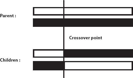
Uniform Crossover: Single bit selected from parent’s string and transferred to the children string.
| Parent | 0 0 0 0 0 0 0 0 0 0 0 0 0 0 0 0 0 0 0 0 0 |
| 1 1 1 1 1 1 1 1 1 1 1 1 1 1 1 1 1 1 1 1 1 | |
| Children | 1 0 1 0 0 1 0 1 0 1 0 0 0 0 0 1 1 1 0 0 1 |
| 0 1 1 0 0 0 1 0 1 0 1 1 0 1 1 0 1 0 0 1 0 |
5.3.2 Standard Genetic Algorithm
Step 1: Create initial population.
Step 2: Estimate fitness of population members.
Step 3: If solution found among member of population, then stop. Otherwise, go to Step 4
Step 4: Select and make copies of individuals.
Step 5: Perform reproduction using crossover and mutation operators. Step 6: Create a new population and go to Step 2.
5.3.3 Genetic Algorithm and Its Application
Researchers and engineers have used genetic algorithm in many applications. By using genetic algorithm, extraordinary and superior outputs and results are achieved. Many literatures are available. Specifically, genetic algorithm is used in energy sector, power system, forecasting, pricing, and many problems.
5.3.4 Power System and Genetic Algorithm
Energy network is a package of energy generation, transmission, and distribution. During these generation, distribution, and transmission, power system struggles from different problems such as economic dispatches, optimal power flow, feeder reconfiguration stability, and many more. In the era of deregulated power system, price forecasting and load forecasting become necessary. In these scenarios, genetic algorithm plays a vital role to solve power system problems. By considering different aspects and constraints such as valve point loading, equality, and inequality, it prohibited operating zone, operating range limit, etc. In the directional search GA, there are two execution of directional search in GA. In first implementation, prohibited operating zones with other constraints have been considered. If all the constraints satisfy for their operating zones, then the attained solution is optimal generation. If any deficiency occurs in units, then set it to the upper or lower limits required. Most GA approaches better compared to other traditional methods and supports maximum unit value [9–16]. The approach cultivates a precise optimal solution for large-scale system [13]. In addition to the losses of the transmission network [14], the adaptability of real coded GA in meeting any number of constraints was also demonstrated by taking into account prohibited operating areas, power balance, and ramp-rate limits. The generating units’ cumulative fuel-cost curves are extremely non-continuous and non-linear inherently. GA is an effective tool for real world problems of optimization. In various fields, it has been used to solve various problems [17]. When finding the high-presentation field, GA is quicker but shows difficulties when local searching for complex problems. This results in premature convergence and also has an unfortunate fine tuning of the final response. GA has been paired with SQP to solve these issues. This approach is used to solve the EDP with incremental fuel-cost functions, considering the valve point results. SQP shows itself as a best non-linear programming method to different optimization problem. The SQP can discover the search space speedily with a gradient direction and assurance a local optimum solution [18]. It is beneficial to advance the presentation of the SQP that the cost function of EDP is approached by using a “smooth and differentiable function” based on the maximum entropy principle [19]. The performance of the results is also compared with [20].
5.3.5 Economic Dispatch Using Genetic Algorithm
Step 1: Randomly created input data as unit data, load demand, etc.
Step 2: Population chromosome initialization.
Step 3: Assess all chromosomes.
Step 4: Rank chromosome rendering to their fitness.
Step 5: Select “best” parents for reproduction.
Step 6: Apply crossover and maybe mutation.
Step 7: Calculate new chromosomes and supplement preeminent into population and displacing weedier chromosomes.
Step 8: If the result converges, otherwise go to Step 5.
5.4 Artificial Neural Network
How does the brain solve all specific aspects in a few milliseconds? This question allows us to create machine vision which initially allows our brain to recognize and process disparate data. The power of our brain can be emphasized by the small size which the smallest supercomputer approaching the processing power of the brain is the size of a football stadium. The work of the human brain is quiet anonymous however some features of this extraordinary mainframe are known. The most basic elements of the human brain are certain cell types that do not seem to regenerate differently from other body parts. It is believed that these cells give us the opportunity to remember, think, and apply past experiences in our every action. One hundred billion of these cells are called neurons. The power of the human mind comes from neurons. Single neurons are complex. They have numerous fragments, sub-systems, and controls. They send data over many electro-chemical paths. Depending on the way used, there are hundreds of different modules of neurons. ANNs are synthetic networks that mimic biological neural networks found in living organisms. In the course of the study, it has been found that there were many differences between architecture and between artificial and natural neural network capabilities. This, in turn, is caused by the limited knowledge shared with the brain. ANNs include ways to regulate synthetic neurons to solve the same difficult and complicated problems that we expect from the so-called human processor the brain. While computers allow for slow and tedious tasks that can be done quickly and accurately compared to human performance, many common tasks are trivial to humans, but formulations that are very difficult to easily complete a computer can. This includes the following:
- Processing signal processing such as image processing, sound processing, and others.
- Data compression.
- Recognition and classification of detection models, including voice and optical character recognition, etc.
- Reconstruction reconstructs and returns data when some data is lost.
- Mining data extraction.
- Simplification of data.
5.4.1 The Biological Neuron
The basic unit of communication of incentive in the nervous system is neurons. Neurons are thought to have three main parts: axons, dendrites, and soma. Soma is part of neurons that contain nucleus, organelle, and cytoplasm. The axon is an extended portion of the nerve where signals (or impulses) travel to the next neuron. Dendrites are small branched projections from catfish that receive impulses from other neurons. Biological neuron is shown in Figure 5.1. When neurons transmit signals to other neurons, signals are transmitted through small spaces called synapses. Synapses act as a gateway between two neurons and connect axons from presynaptic neurons to the dendrites of postsynaptic neurons. The electrical signal produced by presynaptic neurons stimulates the release of chemicals (neurotransmitters) that diffuse through synapses to dendrites and then to soma from postsynaptic neurons. Neurons always maintain potential in their membranes. When postsynaptic neurons receive neurotransmitters, the membrane potential of the neurons changes. When neurons are sufficiently stimulated, the membrane potential near the axons achieves a threshold. After reaching the membrane potential threshold, impulses (potential action) are communicated laterally with the action to the next neuron. Biological neurons can be connected to other neurons and accept connections from other neurons, and therefore, we have a tissue basis. In short, neurons receive information from other neurons, concoct it, and pass that information on to other neurons. Neurons integrate incoming pulses, and when this integration exceeds a certain limit, neurons send pulses in a term. The exact processing that occurs in neurons is unknown.

Figure 5.1 Construction of biological neuron.
5.4.2 A Formal Definition of Neural Network
There is no generally accepted definition of neural networks, i.e., ANNs. But, perhaps most people in the region agree that neural networks are very simple processor networks (“neurons” or “nodes”), each of which has a small amount of local memory. A communication channel connects units that normally transmit numeric data. Nodes only work with their local data and the input they receive via the link. Neural networks are systems that can perform complex calculations, perhaps “intelligent” similar to those routinely carried out by the human brain. Most neural networks “learn” to carry out such intelligent tasks through some form of training, adjusting the weight of the connection based on some training data. In other words, neural networks learn from examples and can generalize outside of training data. In short, neural networks are massively distributed processors that inherently tend to store and expose experienced knowledge to use. In two ways, it looks like a brain: Through the learning process, the network acquires knowledge. The strength of interneuron, called weights, is used to store knowledge gained during training.
5.4.3 Neural Network Models
Mcculloch-Pitts Model
The most uncomplicated model for neurons is the McCulloch-Pitts model, as shown in Figure 5.2. Here, input to neurons is routed through several nodes of the input layer. Inputs are scaled and added by connection weights. Then, the output node produces output by applying the nonlinear function f (.). The three most generally practiced nonlinear functions are the signum, ramp, and sigmoid.
5.4.4 Rosenblatt’s Perceptron
The Rosenblatt basic perceptron model is the same as the single McCulloch-Pitts deviation model, which in this case regulates connection weight through training. The important significance of neural networks lies not only in the way in which neurons are manifested but also in the way in which connections are made (usually referred to as topology). One of the calmest forms of this topology is the multi-layer perceptron, which consists of three layers.
- Input layer (network inputs)
- Hidden layer
- Output layer (network outputs)
There are several layer of neural network. From any one layer, any one neuron is connected to all other neurons in the next layer. This forms of the whole network with fully interconnected. An example of such a network topology is illustrated in Figure 5.3. Inputs (usually digital values) stimulate input levels. Any node can be inserted into the network which can be formulated mathematically. For each input node, this value can be assigned a dissimilar valve liable on the type of input. From all the input nodes, the values are passed to the hidden layer node sideways with the link. The “strength” or “weight” of the link changes the value of the input node by scaling. Each link is given a different weight depending on how important or less important the information presented in this context. The hidden layer node receives information from all connected input nodes [21]. This value, in turn, is passed along with the new link to the output layer in a similar way as the information passed from input to the hidden layer.

Figure 5.2 McCulloch-Pitts model.

Figure 5.3 Multi-layer perceptron structure.
5.4.5 Feedforward and Recurrent Networks
Feedforward and feedback are two main forms of network topology.
Feedforward Network
In a moving neural network, links between units do not form cycles. Feedforward networks generally return very quickly to input. Most cellular networks, in addition to the algorithms invented by neural network researchers, can be trained with various effective conventional numerical methods, such as conjugate and gradients. The network topology for the multilayer perceptron shown above is an example of a simple type of feed-forward network. More complex power grids are made possible by developing the multiple hidden layers.
5.4.6 Back Propagation Algorithm
The backpropagation algorithm is the main central work for continuous work on studying in neural networks. The algorithm instructs to change the weight of the Wpq in each redirection network to learn several partners I/O training. Because the maximum control application uses two-layer MLN, we provide an algorithm for backpropagation. The network is shown in Figure 5.4. x is the n × 1 input vector. y is the m × 1 diagonal output vector. The hidden level consists of unit h, which represents the typical weight connected amongst the source level and the hidden level, while Wjk represents the typical weight connected amongst the hidden level and the input level.
5.4.7 Forward Propagation
The forward response of such a network is given as follows:
jth hidden layer input can be expressed as

Figure 5.4 A two-layered network.
jth hidden layer output can be given as
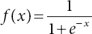
where f is the squashing function, generally taken as sigmoidal activation
Finally ith output layer input is

Output y is given as
Backward Propagation
The instantaneous error wpq of back propagation algorithm is resultant as follows:
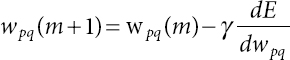
where γ is the learning rate and E = ½ (yd(m) – y (m))2 is the error function to be minimized.
5.4.8 Algorithm
Backpropagation algorithm given as follows:
- Initially, all weights are assigned to random values lies [0, 1].
- Formulate input layer xk, where k =1,2,…, n.
- Signal forwards the propagate through the network using
- Calculate δi for the output layer
Pattern xk is considered by tallying the actual outputs yi with the desired ones

- Calculate the ∆j for the “hidden layers” by propagating the errors backwards
- Update weight as
To update all connection.
- Return back to Step 2 for repetition and to find the next pattern.


5.4.9 Recurrent Network
With feedback or a recurrent neural network, a cycle occurs in connection. In some feedback networks, each moment, an input is offered, a neural network repeats itself long before a response is generated. Feedback networks are more challenging to train than feedforward networks. Figure 5.5 shows the network topology with feedback. Some examples of this type of network are Hopfield models and Boltzmann machines.

Figure 5.5 A recurrent network.
5.4.10 Examples of Neural Networks
The following are few examples of neural networks that perform Boolean logic operations AND, OR, and XOR.
5.4.10.1 AND Operation
The network structure for implementing AND operations with the McCulloch-Pitts model is shown in Figure 5.6. The two input variables a and b are binary values and the third input is a constant called the threshold. Processing the node, labeled τ involves the sum of all inputs to the node and then determining its threshold. The threshold determination node function returns 1 if the summation exceeds zero if not 0. Network input can be mapped into 2D space and the threshold defines the portion of the plane as shown in the figure so that the output on one side is level 1, while the output on the other side is 0, i. H. Airplane is the level of solution. Thresholds must be chosen accordingly. In this case, we take −1.5. Connection weights are all 1.

Figure 5.6 AND network.
5.4.10.2 OR Operation
In Figure 5.7 the OR operation differs from the AND operation only by the position of the decision plane in the 2D inputs space. Therefore, alteration in the threshold value realizes OR operation. Here, we take threshold value equal to −0.5.
5.4.10.3 XOR Operation
However, XOR operation cannot be realized using the simple McCulloch-Pitts model. This is because the outputs here are not linearly separable as in Figure 5.8. It needs two decision planes, and hence, a multiplayer network can only realize the situation. The connection weights, unless otherwise mentioned, are 1. The processing at the hidden and the output nodes, denoted by τ, include summation and thresholding as explained earlier.
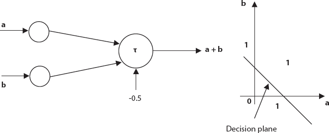
Figure 5.7 OR network.
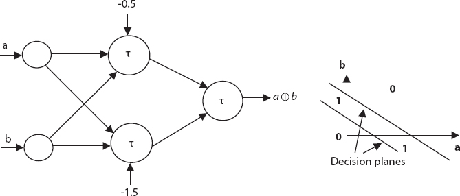
Figure 5.8 XOR network.
5.4.11 Key Components of an Artificial Neuron Network
Each segment describes an artificial neuron network’s seven major components. Both components are efficient when there is one hidden layer in the neural network: one output layer and one input layer at-least.
Segment 1. Weighting Factors: An artificial neural neuron network needs a lot of inputs. Every input has its individual weight which helps to better assess the giving out unit’s “summation function”. These weights have the equal purpose as biology’s neurons. Both inputs are not so efficient and the weights are therefore a superior influence on the processing factor because they converge to generate a neuronal response and provide more value to the effective inputs. In the network, weights are generally termed as adaptive coefficient specifying the amplitude of the artificial neuron input signal. They are a quantity of the connection power of an object. Both abilities can be strengthened through the use of different training systems and the conferral of learning guidelines to a network.
Segment 2. Summation Function: At the start of the process, the weighted sum of all inputs is determined. Inputs and their respective weights are represented arithmetically in the form of a matrix: i1, i2, …, in and w1, w2, …, wn, respectively. As the sum of these two vectors, the whole input signal is represented. The entire signal input function comes from multiply each input I vector component by the corresponding w weight vector component and then summarize all products. Input(1) = i1× w1, input(2) = i2× w2, etc., are added as input(1) + input(2) + … + input(n). The outcome is obtained as a single number, not a vector of multiple components. Geometrically, a measure of their similarity can be called the inner product of two vectors. If the vector is pointing in the same direction, the internal product is maximal if the internal product is considered small, as if the vector is pointing in the 180 degrees out of phase, i.e., opposite direction. The sum function may be more complex than just the number of data sum and weight products. Until switching to the transfer function, multiplying the inputs and calculating the coefficients can be performed in different ways. The addition function may select the minimum, maximum, majority, feature, or some standardization algorithm in addition to simple product addition. The architecture and paradigm of the selected network will determine the basic algorithm to integrate neural inputs. Before it is transferred to the transfer function, several summation functions apply an additional method to the output. This mechanism is sometimes referred to as the “activation function”. “Activation function” is use to permit the final output to change with time. Apparently, the “activation functions” are quite limited to science. Most existing network configurations use an “activation function” called “identity”, which is similar to “not having one”. Moreover, feature is probably to be a section of the entire system rather than just a component of each of the processing unit’s individual components.
Segment 3. Transfer Function: By an algorithmic procedure known as the “transfer function”. The product of the summary function is equal to weighted sum, is transformed into work output. In the transfer function, to evaluate the neuronal output, the summation number can be compared to a certain threshold. If the sum approaches the threshold value, a signal is produced by the processing element. If the input and weight output sum are lesser than the threshold, zero signal or some inhibitory signal is formed. The threshold is commonly non-linear or transition function. Linear functions are constrained as the output is strictly proportional to the input. It is not very good for linear functions. That was the difficulty in the initial models of the network, as stated in the book Perceptrons by Minsky and Papert. Depending on the outcome of the “summation function” is +Ve or −Ve, the transfer function might be something so simple. Zero and one, one and minus one, or other binary variations could be generated by the network. So, a transition function is a “hard limiter” or phase function. Another type of transmission mechanism, the threshold or ramp function, may replicate an area’s input and is still stored as a rigid barrier outside that area. This is a linear function which is set to min and maxvalues, rendering it non-continuous. A sigmoid or S-shaped curve would still be another choice. The curve follows the asymptotes with a minimum and maximum value. This scale is generally referred to as sigmoid if it ranges between −1 and 1 within the range of 0 to 1, an interesting feature of this curve is the continuousness of the mathematical properties and their derivatives. This option works well and is often a transferring selection feature. For different network architectures, other transfer functions have been described and will be conferred future. Before the transfer function is implemented, even circulated arbitrary noise can be introduced. The mode of network paradigm training provided specifies the source and noise level. This noise is usually called artificial neuron “temperature”. The name, “temperature”, comes from the physical phenomenon that affects their ability to think when people become too hot or cold. This method is replicated mechanically by incorporating noise. Indeed, more brain-like transfer functions are evaluated by augmenting disturbance levels to the summation result. To mimic the features of nature more precisely, some experimenters use a source of “Gaussian noise”. “Gaussian noise” is equivalent to randomly dispersed noise although in the temperature range the distribution of random numbers is through a bell curve. Temperature utilization is a field of continuing research and is not used in many technological presentations. “NASA” has just revealed a “network topology” that uses a “temperature coefficient” in a new reproductive training feature. This temperature factor, however, is a worldwide term used to get the function of the gain. This should not be confusing to the more familiar word temperature, simply adding noise to the neurons. In comparison, the “global temperature coefficient” causes the meaning of transmission to have a knowledge variable comparable to the weights of “synaptic input”. This idea is believed to produce a system that has a much higher learning rate (by several orders of magnitudes) than other “feedforward” and “backpropagation networks” and produces more accurate results.
Segment 4. Scaling and Limiting: Completing the transfer feature of the processing unit, the result moves through added processes that scale and restrict. This scaling essentially multiplies the transfer value by averaging a size factor and adding an offset. Limiting is the technique that ensures that no upper or lower bound exceeds the scaled result. This limit is in adding to the hard limits that may have been performed by original transfer function. This method of scaling is used in several configurations to analyze biotic neuron models, namely “brain-state-in- the-box of James Anderson”.
Segment 5. Output Function–Competition: For each processing unit, an output signal is allowed that can be sent to hundreds of other neurons. It is like the biochemical brain, with lots of inputs and just one result. The result is functionally equivalent to the value of the transfer function. Nevertheless, few system configurations change the outcome to accommodate struggle between adjacent processing components. Unless they are strong, neurons can interact with each other, inhibiting processing elements. Competition can occur in one or two stages. Next, the competition will have to decide which artificial neuron or performance will be involved. In addition, competitive feedback helps to assess which factor in development will be involved.
Segment 6. Error Function and Backpropagated Value: In most training grids, there are variations between actual and expected outcomes. This fresh mistake is converted by an “error function” to a specific grid design. Such errors are used by the simplest architecture, but while quadratic error points, cube errors, and other paradigms are retained, they change raw errors to achieve the predefined objectives.
“Artificial neuron error” is usually spread to another processing unit’s learning mechanism. Often the present error is called this type of error. The current error is usually transmitted back to an earlier layer. Nonetheless, this “backpropagated” value may be either the “current error” or the “current error” somehow multiplied.
Segment 7. Learning Function: The learning method aims at modifying variable relationship weights based on a neural algorithm on each unit’s input. This method of regulating the weights of the input connections defined the “adaptation function” and the “learning mode” to achieve some desired results. The learning methods are “supervised” and “unsupervised”. An instructor is required for “supervised learning”. The instructor can be a collection of data training or a viewer who scores the results of the system performance. This method, learning by training, is to have an instructor. When there is no external instructor, certain internal requirements built in the network will structure the program itself. By doing this, it is thinking.
5.4.12 Neural Network Training
A neural network usually has more than two numbers of input nodes and any number of connections between nodes. Once a neural network is built with nodes and some functions to be performed at the nodes, a network can be trained. The networks are trained by changing the weight of links between nodes. Initially, all weights selected randomly. Typically, computer programs generate connection weights at random. The network then receives input and can process information about its node to produce output. Suppose the input is letters and you want from the network to confirm whether the letter “M” or the letter “N”. Primarily, this problem will occur pretty often. The connection weights have to be altered and the network repeat again. Over hundreds of experiments and small variations in connection weights, networks can learn to identify letters very accurately. The whole training setup must be shown multiple times on the network to get satisfying results. Many examples are needed for networks. A common type of neural network training is retransmission. Backward creates a program that automatically changes the link weight if the results are wrong and reinforce the links if the results are correct.
5.4.13 Training Types
Training or learning algorithm can be divided in two parts: (i) Supervised and (ii) Unsupervised.
5.4.13.1 Supervised Training
In the controlled training, the correct result (target value or desired result) is known and communicated to the neural network during exercise so that the neural network can adjust its weight and try to match the results with the target value. After training, it tests the neural network, not the target value, and sees how near it is to get the precise goal value.
5.4.13.2 Unsupervised Training
In case of unsupported training, correct results during training of neural networks are not provided. Unmanaged neural networks usually do some type of data compression, e.g., B. resize or group. The difference between controlled and unsupported methods is always clearly defined. Unsupported methods can study summaries of probability distributions, and these summary distributions can then be used to make predictions.
5.4.14 Learning Rates
The rate of learning from ANNs depends on a number of factors which can be controlled. Many trade-offs need to be considered when choosing the solution. Clearly, a less rate means that much extra period is consumed on off-line learning in order to create a properly trained program. In comparison, with higher learning speeds, a slower learning system could not allow the network to make perfect discrimination possible. Commonly, when addressing the off-line training mission, characterized as “tiresome”, many considerations have to be addressed in addition to time. Network complexity, paradigm range, architecture, learning rule type or rules used, and anticipated correctness need to be taken into consideration. These features play an important role in defining how extended it will take for a network to train. Varying any of these aspects can either prolong the duration of the training to an excessive span or uniform contribute to inappropriate accuracy. Most functions of learning have some facility for a “rate of learning” or “constant learning”. The word is usually positive and varies from zero to one. If the “learning rate” is advanced than one, the learning algorithm can easily override the weight correction. Great rate of “learning” is not precise the prevailing inaccuracies as soon as possible; however, high actions are taken to correct errors, and the best minimum convergence is likely to be reached.
5.4.15 Learning Laws
There are many common applications of learning laws. Most of these rules are some kind of variation in Hebb’s Law, the best recognized and oldest rule of learning. Research into diverse learning mechanisms remains as new ideas surface in commercial journals on a routine basis. Many scholars have the primary objective of modeling biological learning. Some try to adapt their understanding of how nature approaches learning. Any way, it is very minimal that man understands how neural treating essentially works. To be sure, learning is difficult than the simplifications described by the currently defined learning laws. Some of the most important rules are mentioned below.
Hebb’s Rule: Donald Hebb implemented the well-known learning law. The definition appeared in 1949 in his book, “The Organization of Behavior: A Neuropsychological Theory”. His basic rule is: “if a neuron receives an input from another neuron and both are highly active (mathematically having the same sign), the neuron weight should be reinforced.”
Hopfield Law: It is analogous to Hebb’s law, except that it defines the strength or weakening magnitude. It says, “if both the desired output and the input are active or inactive, increase the relation weight by the learning rate, otherwise the learning rate will decrease the weight.”
The Delta Rule: This law is another “Hebb rule” variant. This rule is very popular and most extensively used. The rule is stand on the plain principle of constantly adjusting the input connection intensity to the difference (delta) among the desired output value and the meting out unit’s actual output. To minimalize mean square error, this rule changes the synaptic weight. It is often called as the “Widrow-Hoff Learning Rule” and “Least Mean Square (LMS) Learning Rule”. The Delta method suits in the way such that transfer function derivative converts the delta error in the output layer and is then used to change the input relationship weights in the previous neural layer. In other words, one layer at a time propagates the error back to previous layers. The process of replication of system in accuracies continues until entering the initial layer. The system created is termed as feedforward, and Backpropagation derives its name from this error term computing process. Ensure the input data set is correctly randomized when being used.
The Gradient Descent Rule: This rule is analogous to “delta rules” where the “transfer function” derivative is used to adjust “delta errors” earlier than applying to the ratio weights. Nevertheless, here, an added proportional constant linked to the learning rate is affixed to the weight-acting final amending element. The strategy is extensively applied, although it manages to converge very slowly. Diverse learning stages for diverse level of a network have been shown to help the process of learning converge more quickly. The learning levels for all those near-output layers were set lower in these experiments than near-input layers. The method is particularly vital for users, which is a strong underlying model that does not extract the input data.
Kohonen’s Learning Law: Teuvo Kohonen developed the technique with inspiration of biological systems. The elements strive to evaluate or alter the weighting factor in this method. The processor unit with the highest production is avowed the winner and has the potential to both inhibit its rivals and excite its neighbors. A production is allowed only to the winner and his adjacent are endorsed to change their weights of contact. In addition, during the training period, the size of the vicinity can fluctuate. The normal paradigm is to begin with a broader neighborhood definition and narrow down as the training progression goes on. Kohonen networks are modeling the input distribution according to the idea of the winning variable as the one with the nearby contest to the input prototype. Mentioned thing is useful in modeling numerical or topological data and is often associated with it as maps or topologies that are self-organized.
5.4.16 Restructured Power System
After the invention of ANN, use of ANN has become more important in modern era. Many literatures are available citing ANN applications in medical science, space science, energy system, etc. Here, we discuss ANN application with respect to restructured power system. Since last 25 years, power utility companies are moving toward from monopoly-based system to deregulated system [22]. The electricity market has become more competitive day by day. In restructured power system, different aspects such as transmission congestion management, locational marginal prices, and ancillary service management have become more important. Due to increasing competition, load forecasting and price forecasting become a tedious task for utilities [22].
5.4.17 Advantages of Precise Forecasting of the Price
The correct estimate of the price of electricity helps to create an operative risk management plan for companies contributing in the energy market. At present, market contributors need to use various tools to regulator and diminish risks arising from price volatility in opening markets [23]. If the accuracy comes from the electricity market price, then GENCO and LSE, as the key players, can reduce risk and maximize production. Day time forecasting or hour time forecasting is best example for understanding prediction of forecasting in restructured power system. The power generation from the hydrothermal is considered with “Generation Rate Constraint (GRC)” [24]. “Hybrid Neuro Fuzzy (HNF) controller” is used for testing of control structure. Other effective soft computing techniques are also tested in deregulated power system are “Hybrid Particle Swarm Optimization (HCPSO)”, “Real Coded Genetic Algorithm (RCGA)”, and ANN controllers [25].
5.5 Conclusion
Main objective of chapter was to focus on various soft computing techniques which are based on restructured power system. GA, fuzzy logic, and ANN are major three techniques which are mostly used by electrical engineering researcher. Out of three, neuro fuzzy system is generally used for hybrid system. The widespread application of efficient soft computing techniques is therefore increasing. It has been observed that researcher, those who used SC-based approaches, reported good and positive results, which are encouraging. The main benefit of said approaches is that the results obtained are the clear estimates rather than the unique solution. The techniques described in this chapter assist the end user to take quick decision under the circumstances of uncertainty. The allied areas including science and engineering management are finding soft computing as an essential tool for dealing with the complex problems, and it is very simple to modeling and prediction of the said behavior problems.
References
1. Zadeh, L.A., Fuzzy sets Inf. Control., 8, 3, 338–353, 1965.
2. Yan, H. and Luh, P.B., A Fuzzy Optimization Based Method for Integrated Power System Scheduling and Inter Utility Power Transaction with Uncertainties. IEEE Trans. Power Syst., 12, 2, 756–763, May 1997.
3. Arya, Y., Impact of Hydrogen Aqua Electrolyzer Fuel Cell Units on Auto matic Generation Control of Power Systems with a New Optimal Fuzzy TIDF-II Controller. Renew. Energy, 139, 468–482, 2019.
4. Sabahi, K., Ghaemi, S., Pezeshki, S., Application of Type-2 Fuzzy Logic System for Load Frequency Control using Feedback Error Learning Approaches. Appl. Soft Comput., 21, 1–11, 2014.
5. Arya, Y. and Kumar, N., BFOA-Scaled Fractional Order Fuzzy PID Controller Applied to AGC of Multi Area Multi Source Electric Power Generating Systems. Swarm Evol. Comput., 32, 202–218, 2017.
6. Nanda, J. and Mangla, A., Automatic Generation Control of an Interconnected Hydro-Thermal System using Conventional Integral and Fuzzy Logic Controller. Proceedings of IEEE International Conference on Electric Utility Deregulation, Restructuring and Power Technologies, Hong Kong, China, vol. 1, pp. 372–377, 2004.
7. Chandrashekar, M.J. and Jayapal, R., Design and Comparison of I, PI, PID and Fuzzy Logic Controller on AGC Deregulated Power System with HVDC Link. Proceedings of International Conference on Circuits, Controls and Communications (CCUBE), Bengaluru, pp. 1–6, 2013.
8. Jayapriya, M., Yadav, S., Ram, A.R., Sathvik, S., Lekshmi, R.R., Selva, K.S., Implementation of Fuzzy Based Frequency Stabilization Control Strategy in Raspberry Pi for a Wind Powered Microgrid. Proc. Comput. Sci., 115, 151– 158, 2017.
9. Goldberg, D.E., Genetic Algorithms Search, Optimization & Machine Learning, Addison-Wesley, MA, 1989.
10. Austin, S., An Introduction to Genetic Algorithms, vol. 5, pp. 48–53, Computer Science, March 1990.
11. Chen, P.-H. and Chang, H.-C., Large Scale Economic Dispatch by Genetic Algorithm. IEEE Trans. Power Syst., 10, 4, 1919–1926, 1995.
12. Adhinarayanan, T. and Sydulu, M., A Directional Search Genetic Algorithm to the Economic Dispatch Problem with Prohibited Operating Zones. 2008 IEEE/PES Transmission and Distribution Conference and Exposition, Apr. 21–24, 2008, pp. 1–5.
13. Orero, S.O., Economic dispatch of generators with prohibited operating zones: a genetic algorithm approach. IET Digital Library, 143, 6, 529–534, 1996.
14. Ram Jethmalani, C.H., Simon, S.P., Sundareswaran, K., Srinivasa Rao Nayak, P., Padhy, N.P., Real Coded Genetic Algorithm Based Transmission System Loss Estimation in Dynamic Economic Dispatch Problem. Alex. Eng. J., 57, 3535–3547, 2018.
15. Damousis, I.G., Bakirtzis, A.G., Dokopoulos, P.S., Network-Constrained Economic Dispatch using Real-Coded Genetic Algorithm. IEEE Trans. Power Syst., 18, 1, 198–205, February 2003.
16. Subbaraj, P., Rengaraj, R., Salivahanan, S., Real-Coded Genetic Algorithm Enhanced with Self Adaptation for Solving Economic Dispatch Problem with Prohibited Operating Zone. International Conference on Control, Automation, Communication and Energy Conservation -2009, 4th - 6th June 2009.
17. Luk, P.C.K., Lai, L.L., Tong, T.L., GA Optimisation of Rule Base in a Fuzzy Logic Control of a Solar Power Plant. DRPT2000. International Conference on Electric Utility Deregulation and Restructuring and Power Technologies. Proceedings (Cat. No. 00EX328), 4–7 April 2000, 221–225.
18. He, D.-k., Wang, F.-l., Mao, Z.-z., Hybrid Genetic Algorithm for Economic Dispatch with Valve-Point Effect. Electr. Power Syst. Res., 78, 626–633, 2008.
19. Chiang, C.-L., Improved Genetic Algorithm for Power Economic Dispatch of Units with Valve-Point Effects and Multiple Fuels. IEEE Trans. Power Syst., 20, 4, 1690–1699, November 2005.
20. Tippayachai, J., Ongsakul, W., Ngamroo, I., Parallel Micro Genetic Algorithm for Constrained Economic Dispatch. IEEE Trans. Power Syst., 17, 3, 790–797, August 2002.
21. Podvalnya, S.L. and Vasiljev, E.M., The Principle of Multi-Alternativity in Intelligent Systems: Active Neural Network Models. Proc. Comput. Sci., 103, 410–415, 2017.
22. Xiao, L., Shao, W., Yu, M., Ma, J., Jin, C., Research and Application of A Hybrid Wavelet Neural Network Model with the Improved Cuckoo Search Algorithm for Electrical Power System Forecasting. Appl. Energy, 198, 203– 222, 2017.
23. S, B.S., Kamaraj, N., Hybrid Neuro Fuzzy Approach for Automatic Generation Control in Restructured Power System. Electr. Power Energy Syst., 74, 274– 285, 2016.
24. Shayeghi, H., Shayanfar, H.A., Malik, O.P., Robust Decentralized Neural Networks Based LFC in a Deregulated Power System. Electr. Power Syst. Res., 77, 241–251, 2007.
25. Vahidinasab, V., Jadid, S., Kazemi, A., Day-Ahead Price Forecasting in Restructured Power Systems using Artificial Neural Networks. Electr. Power Syst. Res., 78, 1332–1342, 2008.
- *Corresponding author: [email protected]