CHAPTER 5
TWO-STEP AND MULTISTEP METHODS
The character of some equations, such as the equations of motion in a many-body problem in Newtonian mechanics, requires methods of high and very high orders of accuracy. The use of high-order one-step methods (such as Runge-Kutta methods) for such problems turns out to be computationally very expensive. For this reason multistep methods have been developed. These methods can be both of very high accuracy and fast. In this chapter we study the leapfrog method, which is the simplest of all, and Adams methods, which include both explicit and implicit methods. At the end we show a simple example of the predictor-corrector strategy for multistep methods.
5.1 Multistep methods
Consider the initial value problem
Thus far, we have approximated equation (5.1) by one-step methods (see Definition 2.9). They have the form
If we know vn, we can calculate vn+1. Another class of methods are the multistep methods.1
Definition 5.1 A multistep method to approximate equation (5.1) is of the form
where αj and βj are given constants and r ≥ 1. The method is said to be explicit if β−1 = 0 and implicit otherwise.
The constants αj and βj, which determine a particular method, are chosen to have good accuracy and stability properties.
Notice that to apply a multistep method to the initial value problem (5.1) we set v0 = y0 and then need to prescribe the first r steps v1, v2, …, vr by some supplementary rule, since the iteration needs the previous r + 1 values of vj. This is a drawback of multistep methods compared to one-step methods if during calculation one has to change the step size to maintain the accuracy. In the latter all that is necessary to start the iteration is the initial condition v0 = y0.
Multistep methods are, however, preferred in applications where a very high degree of accuracy is necessary, such as for orbit calculation in many-body problems. The reason is the following. A one-step method would require several evaluations of the function f(v, t) at every time step (e.g., Runge-Kutta methods) or, even worse, evaluations of the function and some of its derivatives (e.g., Taylor methods). On the other hand, a multistep method would require only one evaluation of the function f(v, t) at every time step, because it reuses the evaluations performed in the preceding r + 1 steps. In many applications the evaluation of f(v, t) is by far the most expensive part of the computation; then multistep methods are more efficient.
5.2 Leapfrog method
In this section we consider one particular method, the leapfrog method, which is given by
This method is the explicit two-step method that follows, with r = 1, from (5.3) with α0 = 0, α1 = 1, β−1 = 0, β0 = 2, and β1 = 0, that is, it can be written
It turns out that this method is very efficient for oscillator problems, such as
and also for systems of equations arising from hyperbolic partial differential equations.
The leapfrog method is an example of a two-step method: To compute vn+1, one needs the previous two values, vn and vn-1. In particular, to start the computations one needs v0 and v1. Clearly, if an initial value condition y(0) = y0 is given for (5.2), one can choose v0 = y0. To get v1 one can use the explicit Euler method, for example. Then the starting data for (5.5) are
Exercise 5.1 Why is (5.5), (5.7) second-order accurate?
Truncation error. We will now calculate the truncation error Rn of the leapfrog method. By definition, rn is obtained if one substitutes the exact solution y(t) into the difference equations (5.4). Note that
Therefore,
That is, to leading order the truncation error is ![]() .
.
Stability. To calculate the stability of the leapfrog method, we apply it to the model equation,
![]()
The leapfrog approximation is
Clearly, the solution of (5.8) is determined uniquely by an initial condition
Generalizing Definition 3.6, we define the stability region as follows.
Definition 5.2 The stability region of the leapfrog method consists of all complex numbers λk for which all solutions of (5.8), (5.9) are uniformly bounded for all n = 0, 1, 2, 3, ….
Solutions of difference equations. We first try to find a solution of (5.8) which is of the form
Introducing (5.10) into (5.8) gives us
![]()
Thus, (5.10) is a solution if and only if κ satisfies the so-called characteristic equation
Clearly,
![]()
are solutions of (5.11). Concerning the difference equation (5.5) with initial conditions (5.9), we have to distinguish between two cases.
![]()
![]()
![]()
![]()
Stability region. Since we have computed the general solution of the difference equation (5.8), we can now determine the stability region of the leapfrog method.
Theorem 5.3 The stability region of the leapfrog method consists of all λk with
![]()
Proof: First note that the two points λk = ±i do not belong to the stability region because, by (5.15), the solution of (5.8) is generally unbounded. Now, let λk = ai, a ![]()
![]() , |a| < 1. The roots of the characteristic equation (5.11) are
, |a| < 1. The roots of the characteristic equation (5.11) are
![]()
with |κj|2 = a2 + (1 − a2) = 1. It follows that all solutions of (5.12) remain bounded and the method is stable.
Conversely, assume that λk belongs to the stability region. For the roots κ1,2 of the characteristic equation we have
![]()
Since |κ1| ≤ 1 and |κ2| ≤ 1 we find that |κ1| = |κ2|−1 and then |κ1| = |κ2| = 1. Thus,
![]()
Therefore,
![]()
and the assertion λk = ia, a ![]()
![]() , |a| < 1 follows.
, |a| < 1 follows.
Modified leapfrog method. Since the stability region for the leapfrog method lies on the imaginary axis, one can expect the method to work well for oscillatory problems such as (5.6). For other problems we have to modify it. Consider, for example,
One can approximate (5.16) by
![]()
which is equivalent to
(5.17) ![]()
The modified method is second-order accurate.
Exercise 5.2 Prove that the stability region of the modified leapfrog method (5.16) includes the semiunit disk x2 + y2 < 1, x ≤ 0.
5.3 Adams methods
Definition 5.4 The Adams methods are multistep methods with α0 = 1 and αj = 0 for j = 1, 2, 3, …, r. They are of the form
The constants βj are chosen to get the accuracy and stability properties desired. For example, the Adams-Bashforth are explicit Adams methods; that is, they choose β−1 = 0, and βj with j = 0, 1, …, r so that the accuracy order of the method is as high as possible. It can be shown that an equivalent way to obtain the coefficients is as follows. Integrating equation (5.1) between tn and tn+1 gives
If we replace f(y, t) in the integral by its interpolating polynomial of degree r, at the grid points tn, tn-1, tn-2, …, tn-r, replace y by v as usual, and integrate, we get the Adams-Bashforth method.
Exercise 5.3 Show that the one-step Adams-Bashforth method is just the explicit Euler method and derive the two-step Adams-Bashforth method. Hint: Instead of using the general equation (5.1), use the linear equation dy/dt = λy.
We derive as an example the four-step Adams-Bashforth method, (i.e. with r = 3). It is enough to consider the linear equation dy/dt = λy. Inserting the exact solution into (5.18) and using Taylor expansions centered in yn we see that we can cancel the first four terms of the local error expansion if the following equations are satisfied
These equations have the unique solution β0 = 55/24, β1 = −59/24, β2 = 37/24, and β3 = −3/8, which gives the fourth-order accurate method
In general, the βj, j = 0, 1, …, r, coefficients in a (r + 1)-step Adams-Bashforth method can be chosen to cancel terms in the local error expansion up to ![]() (kr+1). The resulting method is accurate of order r + 1.
(kr+1). The resulting method is accurate of order r + 1.
If one chooses β−1 ≠ 0 in (5.18), on obtains implicit methods called Adams-Moulton methods. In this case one has r + 2 constants to determine and one further term of the local error expansion can be canceled (compared to the Adams-Bashforth methods), thus obtaining an (r + 2)-order accurate method. For example, with a fourth-step Adams-Moulton method we can cancel the first five terms in the local error expansion. The system of equations to satisfy is
whose unique solution is β−1 = 251/720, β0 = 323/360, β1 = −11/30, β2 = 53/360, and β3 = −19/720. The method is fifth-order accurate, given by
(5.22) 
Exercise 5.4 Derive the systems of equations (5.19) and (5.21).
Initial steps. To apply a multistep method one needs to obtain the first r − 1 steps with a different method. A possibility is to use a one-step method of the same order. For example, to apply (5.20), one could compute v1, v2, and v3, applying three steps of the classical fourth-order Runge-Kutta method (3.5).
5.4 Stability of multistep methods
Consider the model problem

Definition 5.5 Multistep method (5.3) is said to be stable if when applied to problem (5.4), the solution vn stays bounded for all n = 0, 1, 2, ….
One can proceed as in the leapfrog method to find solutions of the multistep method. One first looks for solutions of the form vn = κn. Plugging vn into the difference equations (5.3) for the particular problem (5.23) gives
This polynomial equation of degree r + 1 in κ, whose coefficients are linear functions of μ, is sometimes called a characteristic equation. When pμ(κ) has r + 1 distinct roots κj, j = 1, 2, …, r + 1, the general solution of the multi-step method can be written as
In this case the method is clearly stable when |κj| ≤ 1, j = 1, 2, …, r + 1. When some of the roots κj are multiple roots (i.e., have multiplicity greater than 1), some other independent solutions of the form
![]()
are needed to expand the general solution vn. The general solution will be bounded provided that these multiple roots of (5.24) satisfy |κj| < 1. Then we have
Lemma 5.6 The multistep method (5.3) is stable if the solutions κj of (5.24) satisfy
The stability region of the multistep method consists of all the μ in the complex plane such that the method is stable. The fact that all the coefficients of Pμ(κ) are linear functions of μ allows one to apply a simple procedure, known as the boundary locus method, to find the stability region. To understand this method, notice first that pμ(κ) = 0 can be written as
where
By continuity, because of (5.25), for every μ on the boundary of the stability region, at least one of the eigenvalues κj satisfies |κj| = 1. Writing this eigenvalue as κ = eiθ and using (5.26), we have, for the μ on the boundary,
Therefore, to find the boundary of the stability region, one can plot the curve (5.27) for θ ![]() [0, 2π]. This is clearly a closed curve that splits the complex μ-plane in two or more domains. Then, by computing all the roots of pμ(κ) in one arbitrary interior point on every domain to check the condition (5.25), one can identify which of these domains belong to the stability region and which of them do not. Consider, for example, the four-step Adams-Bashforth method (5.20); we have
[0, 2π]. This is clearly a closed curve that splits the complex μ-plane in two or more domains. Then, by computing all the roots of pμ(κ) in one arbitrary interior point on every domain to check the condition (5.25), one can identify which of these domains belong to the stability region and which of them do not. Consider, for example, the four-step Adams-Bashforth method (5.20); we have
![]()
The curve (5.27) divides the complex plane into four domains (see Figure 5.1).
Figure 5.1 Boundary locus for the four-step Adams-Bashforth method.
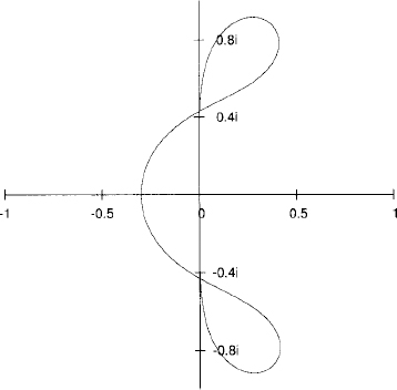
Exercise 5.5 Show that the only domain of Figure 5.1 belonging to the stability region of the four-step Adams-Bashforth method is the one just left of the origin.
Predictor-corrector strategy. In many applications it might be interesting to use implicit multistep methods such as the Adams-Moulton methods introduced earlier. However, the implicit character of these methods implies that one needs to solve large systems of algebraic equations, which become complicated or computationally expensive. A procedure designed to overcome this difficulty is to use an implicit method in combination with an explicit method as a predictor. Here we simply give an example that uses a third-order Adams-Bashforth method as a predictor and a fourth-order Adams-Moulton method as a corrector. If one wants to solve the equation
![]()
this predictor-corrector scheme is
The resulting scheme is clearly explicit.
1Methods of the form (5.3) are sometimes called linear multistep methods, because they use only linear combinations of the values vj and f(vj, tj).