CHAPTER 7
FOURIER SERIES AND INTERPOLATION
Fourier series are among the most useful ideas in mathematics, for many reasons. For the problems we are interested in in this book, Fourier theory is essential to study the stability of numerical approximations and to introduce a family of high-precision methods, the spectral and pseudo-spectral methods. In this chapter we review briefly Fourier series and their ability to represent functions both exactly or as an approximation. We also study Fourier interpolation, which can be thought of as a version of Fourier series for discrete functions.
7.1 Fourier expansion
In this section we consider the expansion of 1-periodic function f(x) into Fourier series. Here f : ![]() →
→ ![]() is called 1-periodic if f(x + 1) = f(x) for all x. Important examples of 1-periodic functions are the exponentials,
is called 1-periodic if f(x + 1) = f(x) for all x. Important examples of 1-periodic functions are the exponentials,
![]()
which play a central role in mathematics. One reason is that differentiation results in multiplication by a constant factor,
![]()
As a consequence, by the use of exponentials, one can often transform a differential equation into an algebraic equation.
For this reason it is important that quite general 1-periodic functions f(x) can be written as Fourier series:
The series converges rapidly if f(x) is smooth.
The complex numbers ![]() (ω) are uniquely determined by f(x). Assuming the representation (7.1), this can be seen as follows. Let ω1 be fixed. Then for all frequencies ω,
(ω) are uniquely determined by f(x). Assuming the representation (7.1), this can be seen as follows. Let ω1 be fixed. Then for all frequencies ω,
(7.3) 
which holds for all frequencies. We call the discrete function ![]() (ω), ω = 0, ±1, ±2, … the Fourier coefficients of f(x).
(ω), ω = 0, ±1, ±2, … the Fourier coefficients of f(x).
By (7.1), we can recover f(x) if we know the Fourier coefficients of f(x). The representation (7.1) is valid if f(x) is only piecewise smooth. Jump discontinuities of f(x) are allowed. However, if f(x) is discontinuous, the convergence is slow.
In the following theorem we state, without proof, some basic results about convergence of Fourier series (see, e.g., [2, 10, 9]).
Definition 7.1 We denote by Cn [a, b] the space of functions that are n times, n ≥ 1, continuously differentiable in the interval a ≤ x ≤ b; and similarly, Cn (a, b) when the interval is a < x < b.
Theorem 7.2 Let f(x) ![]() C1 (−∞, ∞) be 1-periodic. Then the Fourier expansion (7.1) holds and converges uniformly to f(x). If f(x) is only piecewise continuously differentiable, (7.1) converges uniformly in any subinterval [a, b] if f(x)
C1 (−∞, ∞) be 1-periodic. Then the Fourier expansion (7.1) holds and converges uniformly to f(x). If f(x) is only piecewise continuously differentiable, (7.1) converges uniformly in any subinterval [a, b] if f(x) ![]() C1[a, b], while at the points of discontinuity, the Fourier series converges to 1/2(f(x + 0) + f(x − 0)).
C1[a, b], while at the points of discontinuity, the Fourier series converges to 1/2(f(x + 0) + f(x − 0)).
The decay of the Fourier coefficients, as |ω| → ∞, is related to the smoothness of the function; the following theorem is a general result about this.
Lemma 7.3 If f(x) ![]() Cn(−∞, ∞) is 1-periodic, then
Cn(−∞, ∞) is 1-periodic, then
![]()
and
![]()
Proof: For ω = 0 we have
![]()
For ω ≠ O we integrate by parts and note that the contribution from the boundary terms is zero because of the periodicity of f:

that is,
![]()
It is sometimes convenient to work with real quantities If f(x) is a real function, we have
so that the uniqueness of the Fourier coefficients implies that
![]()
or, equivalently,
![]()
Therefore,
The numbers
are real. We have thus obtained an expansion of f(x) in terms of cos(2πωx) and sin(2πωx) with real coefficients.
We illustrate Fourier series with some examples. Consider the piecewise constant, 1-periodic discontinuous function
For ![]() = 0, we obtain
= 0, we obtain
![]()
For ![]() ≠ 0, we have
≠ 0, we have
Thus,
The terms of the series decay only as (2ω + 1)−1 for ω → ∞. Therefore, the convergence of the series is slow.
In Figure 7.1 we plot the approximations of g(x) by the truncated Fourier series
Figure 7.1 g10(x) on the left and g100(x) on the right.

for N = 10 and N = 100. It can be seen in Figure 7.1 that on each side of the jump discontinuity of g(x), the truncated Fourier series gN(x) shows an overshoot or peak that deviates more from the function than it does far from the discontinuity. Moreover, the height of the peak does not seem to go to zero when N increases. In fact, one can show that this peak remains finite in height even in the limit N → ∞. This behavior of Fourier series at jump discontinuities is known as the Gibbs phenomenon.
Exercise 7.1 In this exercise we want to compute the Gibbs phenomenon for the previous example. To this end, compute the height of the first peak (i.e., right to zero and closest to the origin) by finding the maximum of the truncated Fourier series (7.5); you should obtain
Notice that the previous expression can be seen as the midpoint-rule approximation to the integral
![]()
when the interval [0, π] is divided into N + 1 equal subintervals. In the limit N → ∞ the overshoot becomes precisely δ > 0.
If we integrate g(x), we obtain a continuous function
(see Figure 7.2). Integrating the terms of the Fourier series of g(x) gives us
Figure 7.2 Continuous (piecewise smooth) function.

since the constant term is ![]() . We see that the terms in the series decay like (1 + 2ω)−2 as ω → ∞ [i.e. the decay is faster than the series for g(x)].
. We see that the terms in the series decay like (1 + 2ω)−2 as ω → ∞ [i.e. the decay is faster than the series for g(x)].
In Figure 7.3 we show the truncated Fourier series approximating h(x),
Figure 7.3 h1(x) on the left and h10(x) on the right.
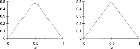
for N = 1 and N = 10. The function h(x) is smoother than g(x) and therefore the Fourier series converges faster.
7.2 L2-norm and scalar product
In the first part of this book we have discussed the fundamental concepts that govern the theory of ordinary differential equations and their numerical solution. The results could often be expressed in terms of estimates in the maximum norm. For time-dependent partial differential equations, in particular for problems of wave propagation, it is much more powerful to express the results in terms of the L2-norm and its scalar product. The reason is that they are often closely related to estimates and concepts of the underlying physics.
They are also connected closely with Fourier expansions which we obtain using the concept of frozen coefficients. In this section we discuss this connection. Let f(x) ![]() C∞(−∞, ∞), g(x)
C∞(−∞, ∞), g(x) ![]() C∞(−∞, ∞) be complex-valued 1-periodic functions. We define the L2-scalar product and norm by
C∞(−∞, ∞) be complex-valued 1-periodic functions. We define the L2-scalar product and norm by
(7.6) ![]()
The scalar product is a bilinear form, that is,
(7.7) 
Also,
(7.8) ![]()
By Lemma 7.3, f, g can be expanded into rapidly converging Fourier series of type (7.1). A fundamental property of Fourier series in relation to the L2-norm and scalar product is
Theorem 7.4 (Parseval’s Relation) If f and g have finite L2-norm, we have
(7.9) 
Proof:
Let f(x) be a piecewise continuous 1-periodic function. Then we can calculate its Fourier coefficients
![]()
For every fixed N, the partial sum
belongs to C∞(−∞, ∞), and by Lemma 7.3 and Theorem 7.4, expression (7.10) can be developed into a rapidly converging Fourier series, satisfying
![]()
We now ask the question: Does fN(x) for N → ∞ converge to f(x) in the L2-norm; that is,
![]()
For our example (7.4), there is no convergence in the maximum norm, because ![]() decays only like
decays only like ![]() .2 However, there is convergence in the L2-norm. We have
.2 However, there is convergence in the L2-norm. We have
A generalization is
Theorem 7.5 Let f(x) be 1-periodic and ![]() its Fourier coefficients. Assume that there are constants K > 0, δ > 1/2 which do not depend on ω such that
its Fourier coefficients. Assume that there are constants K > 0, δ > 1/2 which do not depend on ω such that
![]()
Then f(x) can be developed into a Fourier series and the partial sums fN(x) converge to f(x) in the L2-norm.
In abstract terms one can also express this result in the following way:
![]()
![]()
This process is similar to the one used to define real numbers. In that case we start with rational numbers and add all sequences of rational numbers which are convergent. Of course, we calculate only with rational numbers.
We shall use the same technique and assume that the functions we deal with are C∞-smooth. If not, we approximate them by smooth functions.
7.3 Fourier interpolation
Let f(x) be a smooth 1-periodic function [i.e., f(x) = f(x + 1) for all x]. In Section 7.1 we have shown that we can expand f(x) into a fast-converging Fourier series. Here we want to show that we can interpolate the restriction of f(x) on a grid by a Fourier polynomial.
Let M be a positive integer, h = (2M + 1)−1, a mesh size that defines the grid points xj = jh, j = 0, ± 1, ±2, …. We want to show that we can find interpolation coefficients ![]() (ω) such that the grid function fj = f(xj), j = 0, ±1, ±2, …, is interpolated as
(ω) such that the grid function fj = f(xj), j = 0, ±1, ±2, …, is interpolated as
By assumption, f(xj) is a 1-periodic function on the grid. As
![]()
the same is true for the exponential grid functions in (7.11) and the representation is consistent.
Now we can proceed as in Section 7.1. The interpolation coefficients ![]() (ω) are determined uniquely by the grid values fj, j = 0, 1, 2, …, 2M. This can be seen in the same way as in Section 7.1. By (A. 1) of Section A. 1, the discrete version of (7.2) holds. That is, assuming 0 ≤ ω,
(ω) are determined uniquely by the grid values fj, j = 0, 1, 2, …, 2M. This can be seen in the same way as in Section 7.1. By (A. 1) of Section A. 1, the discrete version of (7.2) holds. That is, assuming 0 ≤ ω, ![]() ≤ 2M, we have
≤ 2M, we have
Let μ be fixed. Then (7.11) and (7.12) give us
Therefore, the interpolation coefficients are given by (7.13).
Fast Fourier transform. It is a remarkable fact that the amount of computational work required to compute the interpolation coefficients is only ![]() (M log M) elementary operations. The corresponding algorithm, which calculates the output
(M log M) elementary operations. The corresponding algorithm, which calculates the output ![]() (ω), − M ≤ ω ≤ M, from the input fj, 0 ≤ j ≤ 2M, is called the fast Fourier transform (FFT). The inverse transformation, which calculates the 2M + 1 grid values fj from the 2M + 1 coefficients
(ω), − M ≤ ω ≤ M, from the input fj, 0 ≤ j ≤ 2M, is called the fast Fourier transform (FFT). The inverse transformation, which calculates the 2M + 1 grid values fj from the 2M + 1 coefficients ![]() (ω), can also be performed in
(ω), can also be performed in ![]() (M log M) operations and is called the inverse fast Fourier transform (IFFT) (see [4, 1]).
(M log M) operations and is called the inverse fast Fourier transform (IFFT) (see [4, 1]).
7.3.1 Scalar product and norm for 1-periodic grid functions
Corresponding to Section 7.2, we introduce a scalar product and norm defined on the space of 1-periodic grid functions (often called l2-scalar product and norm).
Definition 7.6 Let f(xj) = fj, g(xj) = gj be 1-periodic grid functions of type (7.11). The inner product and norm for this grid functions are
(7.14) 
Using (7.11), (7.12) we obtain
Moreover,
Equations (7.15) and (7.16) are a discrete version of Parseval’s relation.
An important property of the Fourier interpolation is that it preserves the smoothness of the original function. We defer a precise statement and proof of this result to Chapter 9, where we discuss discrete approximations to derivatives.
Exercise 7.2 Generalize (7.12) to show that for all integers ω, μ, n,
and therefore (7.13) defines ![]() (μ) for any integer μ. Also show that
(μ) for any integer μ. Also show that
![]()
Exercise 7.3 Let g(x) be the function defined in (7.4). Prove, using finite geometric series, that the interpolation coefficients are
(7.17) ![]()
Exercise 7.4 Consider the discontinuous “sawtooth” 1-periodic function
in the interval x ![]() [0, 1).
[0, 1).
Plot the error eMF(x) = sMF(x) − s(x) separately.
and its error eMI(x) = sMI(x) − s(x).
1The interchange of summation and integration can be justified under quite general assumptions on f. It suffices to assume that ƒ01 |f(x)|2 dx is finite.
2 In this example the convergence can not be uniform since the limit function is discontinuous.