
The K Nearest Neighbors platform predicts a response value based on the responses of the k nearest rows. The k nearest rows to a given row are determined by identifying the k smallest Euclidean distances between the predictor values for that row and the predictor values for each of the other rows. For a continuous response, the predicted value is the average of the responses for the k nearest rows. For a categorical response, the predicted value is the most frequent response level for the k nearest neighbors. If two or more levels are tied as the most frequent levels, the predicted response is assigned by selecting one of these levels at random.
Note: Because ties for most frequent levels in the case of a categorical response are broken at random, results from independent runs of the platform might differ. In a script, add the JSL keyword Nonrandom to the function for a K Nearest Neighbor model to obtain reproducible results.
Each continuous predictor is scaled by its standard deviation. With this scaling, a single predictor with a large range does not excessively influence the distance calculation. Missing values for a continuous predictor are replaced by the mean of that predictor.
Each categorical predictor is expressed in terms of indicator variables, with one indicator variable representing each level. A row with a missing value for a categorical predictor is represented by values of zero on all indicator variables for that predictor.
Note the following potential drawbacks of the k nearest neighbors method:
• K Nearest Neighbors does not make a prediction formula that is practical for large problems.
• K Nearest Neighbors does not produce fitted probabilities for categorical responses.
For more information about the k nearest neighbors method, see Hastie et al. (2009), Hand et al. (2001), and Shmueli et al. (2017).
You have historical financial data for 5,960 customers who applied for home equity loans. Each customer was classified as being a Good Risk or Bad Risk. There is missing data on most of the predictors. You want to construct a model to use in classifying the credit risk of future customers.
1. Select Help > Sample Data and open Equity.jmp.
2. Select Analyze > Predictive Modeling > K Nearest Neighbors.
3. Select BAD and click Y, Response.
Because one of the potential predictors, DEBTINC, has many missing values that might be informative, you do not include it in your model.
4. Select LOAN through CLNO and click X, Factor.
5. Select Validation and click Validation.
6. Click OK.
Figure 8.2 K Nearest Neighbors Report
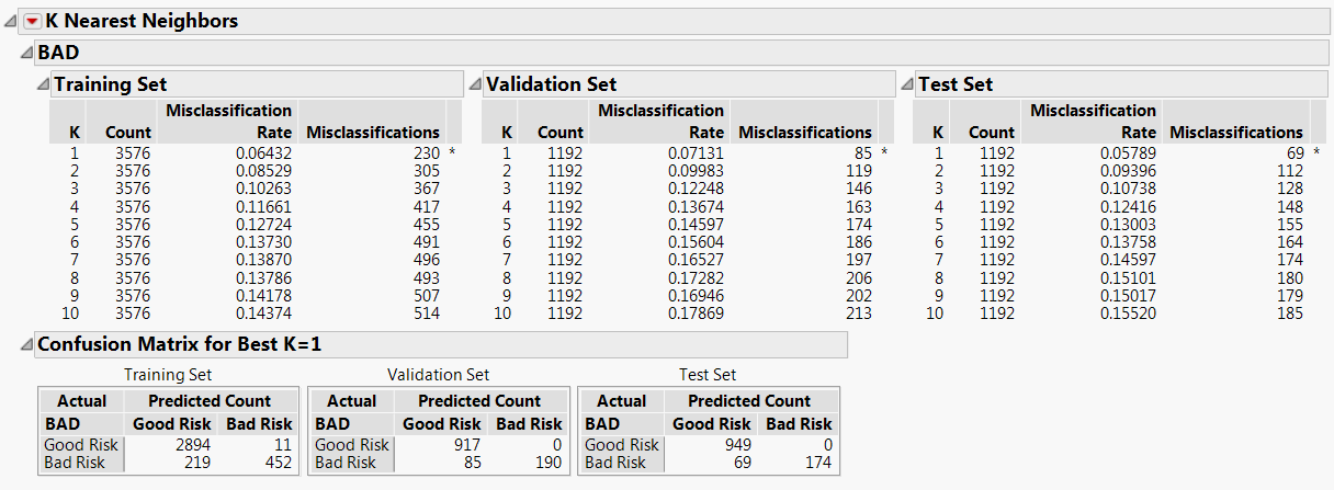
For each value of K, K Nearest Neighbors constructs a model using only the Training Set observations. Each of these models is used to classify the Validation Set observations. In this example, based on the Validation Set results, a model based on the single nearest neighbor (K = 1) has the smallest misclassification rate. The Test Set verifies that the single nearest neighbor model is the best performer for independent data.
7. Click the K Nearest Neighbors red triangle and select Publish Prediction Formula.
8. Next to Number of Neighbors, K, type 1.
This action saves the prediction equation in Formula Depot. Now you can fit other models using other techniques and compare their performance with that of the K = 1 nearest neighbor model using the Model Comparison platform within Formula Depot.
In this example, you want to predict the percent body fat for males using 13 predictors. The Body.jmp sample data table contains percent body fat estimates that are based on underwater weighing and on various body circumference measurements.
1. Select Help > Sample Data Library and open Body Fat.jmp.
2. Select Analyze > Predictive Modeling > K Nearest Neighbors.
3. Select Percent body fat and click Y, Response.
4. Select Age (years) through Wrist circumference (cm) and click X, Factor.
5. Select Validation and click Validation.
6. Click OK.
Figure 8.3 K Nearest Neighbors Report

The K = 8 model had the lowest RMSE for the Validation set. Among k nearest neighbor models, the model based on 8 nearest neighbors seems to perform the best.
Launch the K Nearest Neighbors platform by selecting Analyze > Predictive Modeling > K Nearest Neighbors.
Figure 8.4 K Nearest Neighbors Launch Window

The K Nearest Neighbors launch window provides the following options:
Y, Response
The response variable or variables that you want to analyze.
X, Factor
The predictor variables.
Validation
A numeric column that contains at most three distinct values. See “Validation” in the “Partition Models” chapter.
By
A column or columns whose levels define separate analyses. For each level of the specified column, the corresponding rows are analyzed using the other variables that you have specified. The results are presented in separate reports. If more than one By variable is assigned, a separate report is produced for each possible combination of the levels of the By variables.
Method
Enables you to select the partition method (Decision Tree, Bootstrap Forest, Boosted Tree, K Nearest Neighbors, or Naive Bayes). These alternative methods, except for Decision Tree, are available in JMP Pro.
For more details on these methods, see Chapter 5, “Partition Models”, Chapter 6, “Bootstrap Forest”, Chapter 7, “Boosted Tree”, and Chapter 9, “Naive Bayes”.
Validation Portion
The portion of the data to be used as the validation set. See “Validation” in the “Partition Models” chapter.
Number of Neighbors, K
Maximum number of nearest neighbors to analyze. Models are fit for one nearest neighbor up to the Number of Neighbors, K that you specify.
For each response, the K Nearest Neighbors report is entitled with the name of the response variable and lists information about the models that are fit. The report for the response provides summary information for each of the K models that are fit. The report shows tables for the training set and for the validation and test sets if you defined these using validation.
The statistics reported depend on the modeling type of the response. Each row corresponds to a model defined by K nearest neighbors, where K ranges from one to the value that you specified as Number of Neighbors, K.
An asterisk marks the model for the value K that has the smallest RMSE. The report for a continuous response contains the following columns:
K
Number of nearest neighbors used in the model. K ranges from 1 to the Number of Neighbors, K that you specified in the launch window.
Count
Number of observations used to fit the model.
RMSE
Root mean square error for the model. The model with the smallest RMSE is marked with an asterisk. If there are tied RMSE values, the model with the smallest K is marked with the asterisk.
SSE
Sum of squared errors for the model.
Summary Table
An asterisk marks the model for the value K that has the smallest misclassification rate. The report for a categorical response contains the following columns:
K
Number of nearest neighbors used in the model. K ranges from 1 to the Number of Neighbors, K that you specified in the launch window.
Count
Number of observations used to fit the model.
Misclassification Rate
Proportion of observations misclassified by the model. This is calculated as Misclassifications divided by Count. The model with the smallest misclassification rate is marked with an asterisk. If there are tied misclassification rates, the model with the smallest K is marked with the asterisk.
Misclassifications
Gives the number of observations that are incorrectly predicted by the model.
Confusion Matrix
A confusion matrix is shown for the model with the smallest Misclassification Rate (or the model with the smallest K if there are ties for the smallest misclassification rate). If you use validation, confusion matrices for the validation and test sets appear. A confusion matrix is a two-way classification of actual and predicted responses. Use the confusion matrices and the misclassification rates to guide your selection of a model.
The K Nearest Neighbors red triangle menu contains the following options:
Save Predicteds
Saves K predicted value columns to the data table. The columns are named Predicted <Y, Response> <k>. The kth column contains predictions for the model based on the k nearest neighbors, where Y, Response is the name of the response column.
Save Near Neighbor Rows
Saves K columns to the data table. The columns are named RowNear <k>. For a given row, the kth column contains the row number of its kth nearest neighbor.
Caution: The row numbers in the columns RowNear <k> do not update when you reorder the rows in your data table. If you reorder the rows, the values in those columns are misleading.
Save Prediction Formula
Saves a column that contains a prediction formula for a specific k nearest neighbor model. Enter a value for k when prompted. The prediction formula contains all the training data, so this option might not be practical for large data tables.
Publish Prediction Formula
Creates a prediction formula for the specified k nearest neighbor model and saves it as a formula column script in the Formula Depot platform. If a Formula Depot report is not open, this option creates a Formula Depot report. See the Formula Depot chapter in the Predictive and Specialized Modeling book.
See the JMP Reports chapter in the Using JMP book for more information about the following options:
Local Data Filter
Shows or hides the local data filter that enables you to filter the data used in a specific report.
Redo
Contains options that enable you to repeat or relaunch the analysis. In platforms that support the feature, the Automatic Recalc option immediately reflects the changes that you make to the data table in the corresponding report window.
Save Script
Contains options that enable you to save a script that reproduces the report to several destinations.
Save By-Group Script
Contains options that enable you to save a script that reproduces the platform report for all levels of a By variable to several destinations. Available only when a By variable is specified in the launch window.
..................Content has been hidden....................
You can't read the all page of ebook, please click here login for view all page.