
5 Detecting and Recognizing Faces
Computer vision makes many futuristic-sounding tasks a reality. Two such tasks are face detection (locating faces in an image) and face recognition (identifying a face as belonging to a specific person). OpenCV implements several algorithms for face detection and recognition. These have applications in all sorts of real-world contexts, from security to entertainment.This chapter introduces some of OpenCV's face detection and recognition functionality, along with data files that define particular types of trackable objects. Specifically, in this chapter, we’ll look at Haar cascade classifiers, which analyze the contrast between adjacent image regions to determine whether or not a given image or sub-image matches a known type. We consider how to combine multiple Haar cascade classifiers in a hierarchy so that one classifier identifies a parent region (for our purposes, a face) and other classifiers identify child regions (such as eyes).We also take a detour into the humble but important subject of rectangles. By drawing, copying, and resizing rectangular image regions, we can perform simple manipulations on image regions that we are tracking.We will cover the following topics:
- Understanding Haar cascades
- Finding the pre-trained Haar cascades that come with OpenCV. These include several face detectors
- Using Haar cascades to detect faces in still images and videos
- Gathering images to train and test a face recognizer
- Using several different face recognition algorithms: Eigenfaces, Fisherfaces, and Local Binary Pattern Histograms (LBPHs)
- Copying rectangular regions from one image to another, with or without a mask
- Using a depth camera to distinguish between a face and the background based on depth
- Swapping two people's faces in an interactive application
While this chapter focuses on classic approaches to face detection and recognition, we will go on to explore advanced new models by using OpenCV with a variety of other libraries in Chapter 11, Neutral Networks with OpenCV – an Introduction.
By the end of this chapter, we will have integrated face tracking and rectangle manipulations into Cameo, the interactive application that we have developed in previous chapters. Finally, we will have some face-to-face interaction!
Technical requirements
This chapter uses Python, OpenCV, and NumPy. As part of OpenCV, it uses the optional opencv_contrib modules, which include functionality for face recognition. Some parts of this chapter use OpenCV's optional support for OpenNI 2 to capture images from depth cameras. Please refer back to Chapter 1, Setting Up OpenCV, for installation instructions.The complete code for this chapter can be found in this book's GitHub repository, https://github.com/PacktPublishing/Learning-OpenCV-5-Computer-Vision-with-Python-Fourth-Edition, in the chapter05 folder. Sample images are in the repository images folder.A subset of the chapter’s sample code can be edited and run interactively in Google Colab at https://colab.research.google.com/github/PacktPublishing/Learning-OpenCV-5-Computer-Vision-with-Python-Fourth-Edition/blob/main/chapter05/chapter05.ipynb.
Conceptualizing Haar cascades
When we talk about classifying objects and tracking their location, what exactly are we hoping to pinpoint? What constitutes a recognizable part of an object?Photographic images, even from a webcam, may contain a lot of detail for our (human) viewing pleasure. However, image detail tends to be unstable with respect to variations in lighting, viewing angle, viewing distance, camera shake, and digital noise. Moreover, even real differences in physical detail might not interest us for classification. Joseph Howse, one of this book's authors, was taught in school that no two snowflakes look alike under a microscope. Fortunately, as a Canadian child, he had already learned how to recognize snowflakes without a microscope, as the similarities are more obvious in bulk.Hence, having some means of abstracting image detail is useful in producing stable classification and tracking results. The abstractions are called features, which are said to be extracted from the image data. There should be far fewer features than pixels, though any pixel might influence multiple features. A set of features is represented as a vector (conceptually, a set of coordinates in a multidimensional space), and the level of similarity between two images can be evaluated based on some measure of the distance between the images' corresponding feature vectors.
Later, in Chapter 6, Retrieving Images and Searching Using Image Descriptors, we will explore several kinds of features, as well as advanced ways of describing and matching sets of features.
Haar-like features are one type of feature that is often applied to real-time face detection. They were first used for this purpose in the paper Robust Real-Time Face Detection, by Paul Viola and Michael Jones (International Journal of Computer Vision 57(2), 137–154, Kluwer Academic Publishers, 2001). An electronic version of this paper is available at http://comp3204.ecs.soton.ac.uk/cw/viola04ijcv.pdf.Each Haar-like feature describes the pattern of contrast among adjacent image regions. For example, edges, vertices, and thin lines each generate a kind of feature. Some features are distinctive in the sense that they typically occur in a certain class of object (such as a face) but not in other objects. These distinctive features can be organized into a hierarchy, called a cascade, in which the highest layers contain features of greatest distinctiveness, enabling a classifier to quickly reject subjects that lack these features. If a subject is a good match for the higher-layer features, then the classifier considers the lower-layer features too in order to weed out more false positives.For any given subject, the features may vary depending on the scale of the image and the size of the neighborhood (the region of nearby pixels) in which contrast is being evaluated. The neighborhood’s size is called the window size. To make a Haar cascade classifier scale-invariant or, in other words, robust to changes in scale, the window size is kept constant but images are rescaled a number of times; hence, at some level of rescaling, the size of an object (such as a face) may match the window size. Together, the original image and the rescaled images are called an image pyramid, and each successive level in this pyramid is a smaller rescaled image. OpenCV provides a scale-invariant classifier that can load a Haar cascade from an XML file in a particular format. Internally, this classifier converts any given image into an image pyramid.Haar cascades, as implemented in OpenCV, are not robust to changes in rotation or perspective. For example, an upside-down face is not considered similar to an upright face and a face viewed in profile is not considered similar to a face viewed from the front. A more complex and resource-intensive implementation could improve a Haar cascade’s robustness to rotation by considering multiple transformations of images as well as multiple window sizes. However, we will confine ourselves to the implementation in OpenCV.
Getting Haar cascade data
Your installation of OpenCV 5 should contain a subfolder called data. The path to this folder is stored in an OpenCV variable called cv2.data.haarcascades.The data folder contains XML files that can be loaded by an OpenCV class called cv2.CascadeClassifier. An instance of this class interprets a given XML file as a Haar cascade, which provides a detection model for a type of object such as a face. cv2.CascadeClassifier can detect this type of object in any image. As usual, we could obtain a still image from a file, or we could obtain a series of frames from a video file or a video camera.From the data folder, we will use the following cascade files:
haarcascade_frontalface_default.xml
haarcascade_eye.xml
As their names suggest, these cascades are for detecting faces and eyes. They require a frontal, upright view of the subject. We will use them later when building a face detector.
If you are curious about how these cascade files are generated, you can find more information in Joseph Howse's book, OpenCV 4 for Secret Agents (Packt Publishing, 2019), specifically in Chapter 3, Training a Smart Alarm to Recognize the Villain and His Cat. With a lot of patience and a reasonably powerful computer, you can make your own cascades and train them for various types of objects.
Using OpenCV to perform face detection
With cv2.CascadeClassifier, it makes little difference whether we perform face detection on a still image or a video feed. The latter is just a sequential version of the former: face detection on a video is simply face detection applied to each frame. Naturally, with more advanced techniques, it would be possible to track a detected face continuously across multiple frames and determine that the face is the same one in each frame. However, it is good to know that a basic sequential approach also works.Let's go ahead and detect some faces.
Performing face detection on a still image
The first and most basic way to perform face detection is to load an image and detect faces in it. To make the result visually meaningful, we will draw rectangles around faces in the original image. Remembering that the face detector is designed for upright, frontal faces, we will use an image of a row of people, specifically woodcutters, standing shoulder to shoulder and facing the photographer or viewer.Let's go ahead and create the following basic script to perform face detection:
import cv2face_cascade = cv2.CascadeClassifier(
    f'{cv2.data.haarcascades}haarcascade_frontalface_default.xml')
img = cv2.imread('../images/woodcutters.jpg')
gray = cv2.cvtColor(img, cv2.COLOR_BGR2GRAY)
faces = face_cascade.detectMultiScale(gray, 1.08, 5)
for (x, y, w, h) in faces:
    img = cv2.rectangle(img, (x, y), (x+w, y+h), (255, 255255, 0), 2)

cv2.namedWindow('Woodcutters Detected!')
cv2.imshow('Woodcutters Detected!', img)
cv2.imwrite('./woodcutters_detected.pngpng', img)
cv2.waitKey(0)
Let's walk through the preceding code in small steps. First, we use the obligatory cv2 import that you will find in every script in this book. Then, we declare a face_cascade variable, which is a CascadeClassifier object that loads a cascade for face detection:
face_cascade = cv2.CascadeClassifier(
    f'{cv2.data.haarcascades}haarcascade_frontalface_default.xml')
We then load our image file with cv2.imread and convert it into grayscale because CascadeClassifier, like many of OpenCV’s classifiers, expects grayscale images. (If we try to use a color image, CascadeClassifier will internally convert it to grayscale anyway.) The next step, face_cascade.detectMultiScale, is where we perform the actual face detection:
img = cv2.imread('../images/woodcutters.jpg')
gray = cv2.cvtColor(img, cv2.COLOR_BGR2GRAY)
faces = face_cascade.detectMultiScale(gray, 1.08, 5)
The parameters of detectMultiScale include scaleFactor and minNeighbors. The scaleFactor argument, which should be greater than 1.0, determines the downscaling ratio of the image at each iteration of the face detection process. As we discussed earlier in the Conceptualizing Haar cascades section, this downscaling is intended to achieve scale invariance by matching various faces to the window size. The minNeighbors argument is the minimum number of overlapping detections that are required in order to retain a detection result. Normally, we expect that a face may be detected in multiple overlapping windows, and a greater number of overlapping detections makes us more confident that the detected face is truly a face.The value returned from the detection operation is a list of tuples that represent the face rectangles. OpenCV's cv2.rectangle function allows us to draw rectangles at the specified coordinates. x and y represent the left and top coordinates, while w and h represent the width and height of the face rectangle. We draw cyan rectangles around all of the faces we find by looping through the faces variable, making sure we use the original image for drawing, not the gray version:
for (x, y, w, h) in faces:
    cv2.rectangle(img, (x, y), (x+w, y+h), (255, 255255, 0), 2)
Lastly, we call cv2.imshow to display the resulting processed image and we call cv2.imwrite to save it. As usual, to prevent the image window from closing automatically, we insert a call to waitKey, which returns when the user presses any key:
cv2.imshow('Woodcutters Detected!', img)
cv2.imwrite('./woodcutters_detected.pngpng', img)
cv2.waitKey(0)
And there we go, three members of the band of woodcutters have been detected in our image, as shown in the following screenshot:
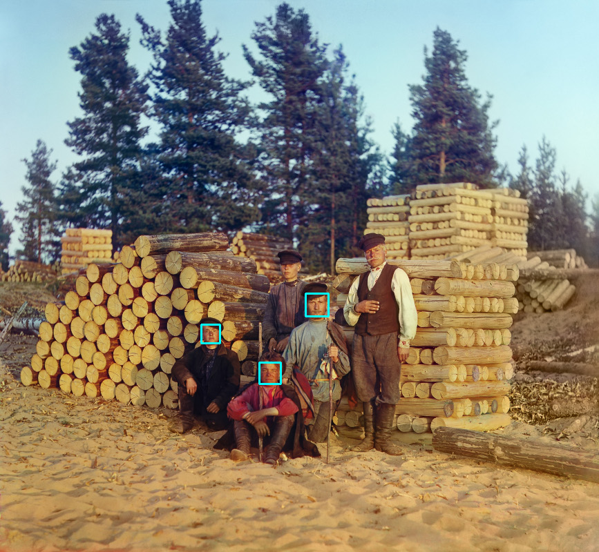
The photograph in this example is the work of Sergey Prokudin-Gorsky (1863-1944), a pioneer of color photography. Tsar Nicholas II sponsored Prokudin-Gorsky to photograph people and places throughout the Russian Empire as a vast documentary project. Prokudin-Gorsky photographed these woodcutters near the Svir river, in northwestern Russia, in 1909.
Here, we have no false positive detections; all three rectangles really are woodcutters’ faces. However, we do have two false negatives (woodcutters whose faces were not detected). Try adjusting the parameters of face_cascade.detectMultiScale to see how the results change. Then, let’s proceed to a more interactive example.
Performing face detection on a video
We now understand how to perform face detection on a still image. As mentioned previously, we can repeat the process of face detection on each frame of a video (be it a camera feed or a pre-recorded video file).The next script will open a camera feed, read a frame, examine that frame for faces, and scan for eyes within the detected faces. Finally, it will draw blue rectangles around the faces and green rectangles around the eyes. Here is the script in its entirety:
import cv2
face_cascade = cv2.CascadeClassifier(
    f'{cv2.data.haarcascades}haarcascade_frontalface_default.xml')
eye_cascade = cv2.CascadeClassifier(
    f'{cv2.data.haarcascades}haarcascade_eye.xml')
camera = cv2.VideoCapture(0)
while (cv2.waitKey(1) == -1):
    success, frame = camera.read()
    if success:
        gray = cv2.cvtColor(frame, cv2.COLOR_BGR2GRAY)
        faces = face_cascade.detectMultiScale(
            gray, 1.3, 5, minSize=(120, 120))
        for (x, y, w, h) in faces:
            cv2.rectangle(frame, (x, y), (x+w, y+h), (255, 0, 0), 2)
            roi_gray = gray[y:y+h, x:x+w]
            eyes = eye_cascade.detectMultiScale(
                roi_gray, 1.11, 5, minSize=(40, 40))
            for (ex, ey, ew, eh) in eyes:
                cv2.rectangle(frame, (x+ex, y+ey),
                              (x+ex+ew, y+ey+eh), (0, 255, 0), 2)
        cv2.imshow('Face Detection', frame)
Let's break up the preceding sample into smaller, more digestible chunks:
- As usual, we import the
cv2module. After that, we initialize twoCascadeClassifierobjects, one for faces and another for eyes:
face_cascade = cv2.CascadeClassifier(    f'{cv2.data.haarcascades}haarcascade_frontalface_default.xml')
eye_cascade = cv2.CascadeClassifier(
f'{cv2.data.haarcascades}haarcascade_eye.xml')- As in most of our interactive scripts, we open a camera feed and start iterating over frames. We continue until the user presses any key. Whenever we successfully capture a frame, we convert it into grayscale as our first step in processing it:
camera = cv2.VideoCapture(0)
while (cv2.waitKey(1) == -1):
    success, frame = camera.read()
    if success:
gray = cv2.cvtColor(frame, cv2.COLOR_BGR2GRAY)- We detect faces with the
detectMultiScalemethod of our face detector. As we have previously done, we use thescaleFactorandminNeighborsarguments. We also use theminSizeargument to specify a minimum size of a face, specifically 120x120. No attempt will be made to detect faces smaller than this. (Assuming that our user is sitting close to the camera, it is safe to say that the user's face will be larger than 120x120 pixels.) Here is the call todetectMultiScale:
faces = face_cascade.detectMultiScale(
gray, 1.3, 5, minSize=(120, 120))- We iterate over the rectangles of the detected faces. We draw a blue border around each rectangle in the original color image. Then, within the same rectangular region of the grayscale image, we perform eye detection:
for (x, y, w, h) in faces:
    cv2.rectangle(frame, (x, y), (x+w, y+h), (255, 0, 0), 2)
    roi_gray = gray[y:y+h, x:x+w]
    eyes = eye_cascade.detectMultiScale(
        roi_gray, 1.1, 5, minSize=(40, 40))
The eye detector is a bit less accurate than the face detector. You might see shadows, parts of the frames of glasses, or other regions of the face falsely detected as eyes. To improve the results, you could try defining
roi_grayas a smaller region of the face, since we can make a good guess about the eyes' location in an upright face. You could also try using amaxSizeargument to avoid false positives that are too large to be eyes. Also, you could adjustminSizeandmaxSizeso that the dimensions are proportional towandh, the size of the detected face. As an exercise, feel free to experiment with changes to these and other parameters.
- We loop through the resulting eye rectangles and draw green outlines around them:
for (ex, ey, ew, eh) in eyes:
    cv2.rectangle(frame, (x+ex, y+ey),
(x+ex+ew, y+ey+eh), (0, 255, 0), 2)- Finally, we show the resulting frame in the window:
cv2.imshow('Face Detection', frame)Run the script. If our detectors produce accurate results, and if any face is within the field of view of the camera, you should see a blue rectangle around the face and a green rectangle around each eye, as shown in this screenshot:

Experiment with this script to see how the face and eye detectors perform under various conditions. Try a brighter or darker room. If you wear glasses, try removing them. Try various people's faces and various expressions. Adjust the detection parameters in the script to see how they affect the results. When you are satisfied, let's consider what else we can do with faces in OpenCV.
Performing face recognition
Detecting faces is a fantastic feature of OpenCV and one that constitutes the basis for a more advanced operation: face recognition. What is face recognition? It is the ability of a program, given an image or a video feed containing a person's face, to identify that person. One of the ways to achieve this (and the approach adopted by OpenCV) is to train the program by feeding it a set of classified pictures (a facial database) and perform recognition based on the features of those pictures.Another important feature of OpenCV's face recognition module is that each recognition has a confidence score, which allows us to set thresholds in real-life applications to limit the incidence of false identifications.Let's start from the very beginning; to perform face recognition, we need faces to recognize. We fulfill this requirement in two ways: supply the images ourselves or obtain freely available face databases. A large directory of face databases is available online at http://www.face-rec.org/databases/. Here are a few notable examples from the directory:
- Yale Face Database (Yalefaces): http://vision.ucsd.edu/content/yale-face-database
- Extended Yale Face Database B: http://vision.ucsd.edu/content/extended-yale-face-database-b-b
- Database of Faces (from AT&T Laboratories Cambridge): https://cam-orl.co.uk/facedatabase.html
If we trained a face recognizer on these samples, we would then have to run face recognition on an image that contains the face of one of the sampled people. This process might be educational, but perhaps not as satisfying as providing images of our own. You probably had the same thought that many computer vision learners have had: I wonder if I can write a program that recognizes my face with a certain degree of confidence. Indeed, you can and soon you will!
Generating the data for face recognition
Let's go ahead and write a script that will generate those images for us. A few images containing different expressions are all that we need, but it is preferable that the training images are square and are all the same size. Our sample script uses a size of 200x200, but most freely available datasets have smaller images than this.Here is the script itself:
import cv2
import os
output_folder = '../data/at/jm'
if not os.path.exists(output_folder):
    os.makedirs(output_folder)
face_cascade = cv2.CascadeClassifier(
    f'{cv2.data.haarcascades}haarcascade_frontalface_default.xml')
camera = cv2.VideoCapture(0)
count = 0
while (cv2.waitKey(1) == -1):
    success, frame = camera.read()
    if success:
        gray = cv2.cvtColor(frame, cv2.COLOR_BGR2GRAY)
        faces = face_cascade.detectMultiScale(
            gray, 1.3, 5, minSize=(120, 120))
        for (x, y, w, h) in faces:
            cv2.rectangle(frame, (x, y), (x+w, y+h), (255, 0, 0), 2)
            face_img = cv2.resize(gray[y:y+h, x:x+w], (200, 200))
            face_filename = '%s/%d.pgm' % (output_folder, count)
            cv2.imwrite(face_filename, face_img)
            count += 1
        cv2.imshow('Capturing Faces...', frame)
Here, we are generating sample images by building on our newfound knowledge of how to detect a face in a video feed. We are detecting a face, cropping that region of the grayscale-converted frame, resizing it to be 200x200 pixels, and saving it as a PGM file with a name in a particular folder (in this case, jm, one of the authors’ initials; you can use your own initials). Like many of our windowed applications, this one runs until the user presses any key.The count variable is present because we needed progressive names for the images. Run the script for a few seconds, change your facial expression a few times, and check the destination folder you specified in the script. You will find a number of images of your face, grayed, resized, and named with the format <count>.pgm.Modify the output_folder variable to make it match your name. For example, you might choose '../data/at/my_name'. Run the script, wait for it to detect your face in a number of frames (say, 20 or more), and then press any key to quit. Now, modify the output_folder variable again to make it match the name of a friend whom you also want to recognize. For example, you might choose '../data/at/name_of_my_friend'. Do not change the base part of the folder (in this case, '../data/at') because later, in the Loading the training data for face recognition section, we will write code that loads the training images from all of the subfolders of this base folder. Ask your friend to sit in front of the camera, run the script again, let it detect your friend's face in a number of frames, and then quit. Repeat this process for any additional people you might want to recognize.Let's now move on to try and recognize the user's face in a video feed. This should be fun!
Choosing a face recognition algorithm
OpenCV 5 implements three different algorithms for recognizing faces: Eigenfaces, Fisherfaces, and Local Binary Pattern Histograms (LBPHs). Eigenfaces and Fisherfaces are derived from a more general-purpose algorithm called Principal Component Analysis (PCA). For a detailed description of the algorithms, refer to the following links:
- PCA: A Tutorial on Principal Component Analysis (2013), by Jonathon Shlens, is available at http://arxiv.org/pdf/1404.1100v1.pdf. This algorithm was invented in 1901 by Karl Pearson, and the original paper, On Lines and Planes of Closest Fit to Systems of Points in Space, is available at http://pca.narod.ru/pearson1901.pdf.
- Eigenfaces: The paper Eigenfaces for Recognition (1991), by Matthew Turk and Alex Pentland, is available at http://www.cs.ucsb.edu/~mturk/Papers/jcn.pdf.
- Fisherfaces: The seminal paper The Use of Multiple Measurements in Taxonomic Problems (1936), by R. A. Fisher, is available at http://onlinelibrary.wiley.com/doi/10.1111/j.1469-1809.1936.tb02137.x/pdf.
- Local Binary Pattern: The first paper describing this algorithm is Performance evaluation of texture measures with classification based on Kullback discrimination of distributions (1994), by T. Ojala, M. Pietikainen, and D. Harwood. It is available at https://ieeexplore.ieee.org/document/576366.
For this book's purposes, let's just take a high-level overview of the algorithms. First and foremost, they all follow a similar process; they take a set of classified observations (our face database, containing numerous samples per individual), train a model based on it, perform an analysis of face images (which may be face regions that we detected in an image or video), and determine two things: the subject's identity and a measure of confidence that this identification is correct. The latter is commonly known as the confidence score.Eigenfaces performs PCA, which identifies principal components of a certain set of observations (again, your face database), calculates the divergence of the current observation (the face being detected in an image or frame) compared to the dataset, and produces a value. The smaller the value, the smaller the difference between the face database and the detected face; hence, a value of 0 is an exact match.Fisherfaces also derives from PCA and evolves the concept, applying more complex logic. While computationally more intensive, it tends to yield more accurate results than Eigenfaces.LBPH instead divides a detected face into small cells and, for each cell, builds a histogram that describes whether the brightness of the image is increasing when comparing neighboring pixels in a given direction. This cell's histogram can be compared to the histogram of the corresponding cell in the model, producing a measure of similarity. Of the face recognizers in OpenCV, the implementation of LBPH is the only one that allows the model sample faces and the detected faces to be of a different shape and size. Hence, it is a convenient option, and the authors of this book find that its accuracy compares favorably to the other two options.Despite the algorithms’ differences, OpenCV provides a similar interface for all three, as we shall soon see.
Loading the training data for face recognition
Regardless of our choice of face recognition algorithm, we can load the training images in the same way. Earlier, in the Generating the data for face recognition section, we generated training images and saved them in folders that were organized according to people's names or initials. For example, the following folder structure could contain sample face images of this book's authors, Joseph Howse (jh) and Joe Minichino (jm):
../
  data/
    at/
      jh/
      jm/
Let's write a script that loads these images and labels them in a way that OpenCV's face recognizers will understand. To work with the filesystem and the data, we will use the Python standard library's os module, as well as the cv2 and numpy modules. Let's create a script that starts with the following import statements:
import os
import cv2
import numpy
Let's add the following read_images function, which walks through a directory's subdirectories, loads the images and shows each of them for user information purposes, resizes them to a specified size, and puts the resized images in a list. The order of this list has no significance in itself but, at the same time, our function builds two corresponding lists that describe the images: first, a corresponding list of people's names or initials (based on the subfolder names), and second, a corresponding list of labels or numeric IDs associated with the loaded images. For example, jh could be a name and 0 could be the label for all images that were loaded from the jh subfolder. Finally, the function converts the lists of images and labels into NumPy arrays, and it returns three variables: the list of names, the NumPy array of images, and the NumPy array of labels. Here is the function's implementation:
def read_images(path, image_size):
    names = []
    training_images, training_labels = [], []
    label = 0
    for dirname, subdirnames, filenames in os.walk(path):
        for subdirname in subdirnames:
            names.append(subdirname)
            subject_path = os.path.join(dirname, subdirname)
            for filename in os.listdir(subject_path):
                img = cv2.imread(os.path.join(subject_path, filename),
                                 cv2.IMREAD_GRAYSCALE)
                if img is None:
                    # The file cannot be loaded as an image.
                    # Skip it.
                    continue
                img = cv2.resize(img, image_size)
                cv2.imshow('training', img)
                cv2.waitKey(5)
                training_images.append(img)
                training_labels.append(label)
            label += 1
    training_images = numpy.asarray(training_images, numpy.uint8)
    training_labels = numpy.asarray(training_labels, numpy.int32)
    return names, training_images, training_labels
Let's call our read_images function by adding code such as the following:
path_to_training_images = '../data/at'
training_image_size = (200, 200)
names, training_images, training_labels = read_images(
    path_to_training_images, training_image_size)
Edit the
path_to_training_imagesvariable in the preceding code block to ensure that it matches the base folder of theoutput_foldervariables you defined earlier in the code for the section Generating the data for face recognition.
So far, we have training data in a useful format but we have not yet created a face recognizer or performed any training. We will do so in the next section, where we continue the implementation of the same script.
Performing face recognition with Eigenfaces
Now that we have an array of training images and an array of their labels, we can create and train a face recognizer with just two more lines of code:
model = cv2.face.EigenFaceRecognizer_create()
model.train(training_images, training_labels)
What have we done here? We created the Eigenfaces face recognizer with OpenCV's cv2.EigenFaceRecognizer_create function, and we trained the recognizer by passing the arrays of images and labels (numeric IDs). Optionally, we could have passed two arguments to cv2.EigenFaceRecognizer_create:
num_components: This is the number of components to keep for the PCA.threshold: This is a floating-point value specifying a confidence threshold. Faces with a confidence score below the threshold will be discarded. By default, the threshold is the maximum floating-point value so that no faces are discarded.
Having trained this model, we could save it to a file using code such as
model.write('my_model.xml'). Later (for example, in another script), we could skip the training step and just load the pre-training model from the file using code such asmodel.read('my_model.xml'). However, for the sake of our simple demo, we will just train and test the model in one script without saving the model to a file.
To test this recognizer, let's use a face detector and a video feed from a camera. As we have done in previous scripts, we can use the following line of code to initialize the face detector:
face_cascade = cv2.CascadeClassifier(
    f'{cv2.data.haarcascades}haarcascade_frontalface_default.xml')
The following code initializes the camera feed, iterates over frames (until the user presses any key), and performs face detection and recognition on each frame:
camera = cv2.VideoCapture(0)
while (cv2.waitKey(1) == -1):
success, frame = camera.read()
if success:
faces = face_cascade.detectMultiScale(frame, 1.3, 5)
for (x, y, w, h) in faces:
cv2.rectangle(frame, (x, y), (x+w, y+h), (255, 0, 0), 2)
gray = cv2.cvtColor(frame, cv2.COLOR_BGR2GRAY)
roi_gray = gray[x:x+w, y:y+h]
if roi_gray.size == 0:
# The ROI is empty. Maybe the face is at the image edge.
# Skip it.
continue
roi_gray = cv2.resize(roi_gray, training_image_size)
label, confidence = model.predict(roi_gray)
text = '%s, confidence=%.2f' % (names[label], confidence)
cv2.putText(frame, text, (x, y - 20),
cv2.FONT_HERSHEY_SIMPLEX, 1, (255, 0, 0), 2)
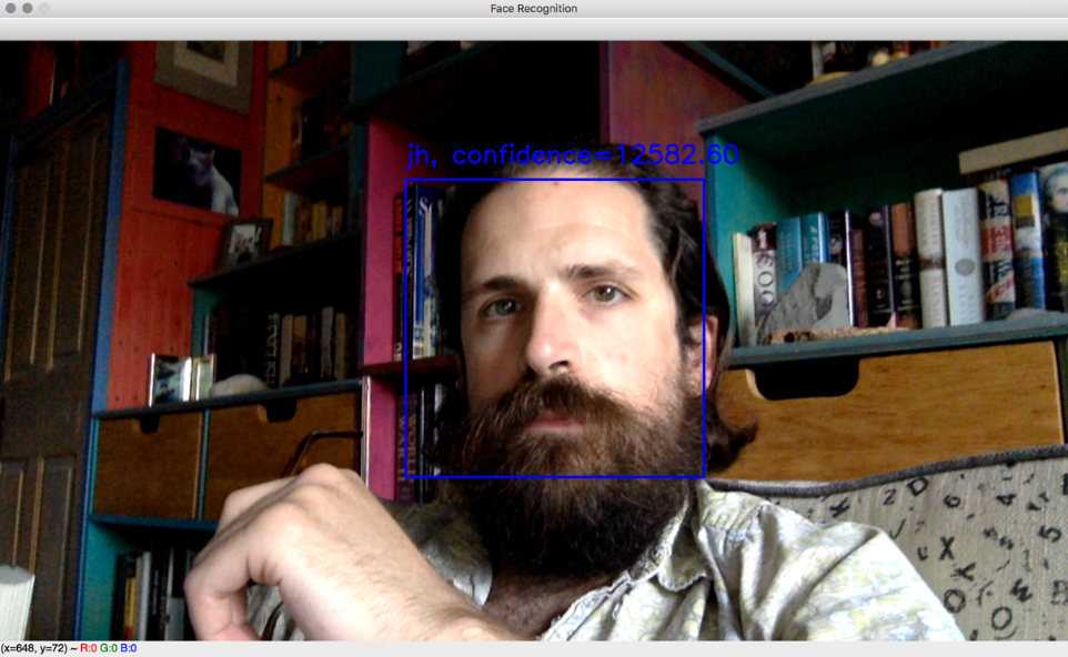
cv2.imshow('Face Recognition', frame)Let's walk through the most important functionality of the preceding block of code. For each detected face, we convert and resize it so that we have a grayscale version that matches the expected size (in this case, 200x200 pixels as defined by the training_image_size variable in the previous section, Loading the training data for face recognition). Then, we pass the resized, grayscale face to the face recognizer's predict function. This returns a label and confidence score. We look up the person's name corresponding to the numeric label of that face. (Remember that we created the names array in the previous section, Loading the training data for face recognition.) We draw the name and confidence score in blue text above the recognized face. After iterating over all detected faces, we display the annotated image.
We have taken a simple approach to face detection and recognition, and it serves the purpose of enabling you to have a basic application running and understand the process of face recognition in OpenCV 5. To improve upon this approach and make it more robust, you could take further steps such as correctly aligning and rotating detected faces so that the accuracy of the recognition is maximized.
When you run the script, you should see something similar to the following screenshot:
Next, let's consider how we would adapt these script to replace Eigenfaces with another face recognition algorithm.
Performing face recognition with Fisherfaces
What about Fisherfaces? The process does not change much; we simply need to instantiate a different algorithm. With default arguments, the declaration of our model variable would look like this:
model = cv2.face.FisherFaceRecognizer_create()cv2.face.FisherFaceRecognizer_create takes the same two optional arguments as cv2.createEigenFaceRecognizer_create: the number of principal components to keep and the confidence threshold. As you might guess, these types of *_create functions are quite common in OpenCV for situations where several different algorithms share a common interface. Let’s look at one more example.
Performing face recognition with LBPH
For the LBPH algorithm, again, the process is similar. However, the algorithm factory takes the following optional parameters (in order):
radius: The pixel distance between the neighbors that are used to calculate a cell's histogram (by default, 1)neighbors: The number of neighbors used to calculate a cell's histogram (by default, 8)grid_x: The number of cells into which the face is divided horizontally (by default, 8)grid_y: The number of cells into which the face is divided vertically (by default, 8)confidence: The confidence threshold (by default, the highest possible floating-point value so that no results are discarded)
With default arguments, the model declaration would look like this:
model = cv2.face.LBPHFaceRecognizer_create() Note that, with LBPH, we do not need to resize images as the division into grids allows a comparison of patterns identified in each cell.
Having looked at the available face recognition algorithms, let’s now consider how to evaluate a recognition result.
Discarding results based on the confidence score
The predict method returns a tuple, in which the first element is the label of the recognized individual and the second is the confidence score. All algorithms come with the option of setting a confidence score threshold, which measures the distance of the recognized face from the original model; therefore, a score of 0 signifies an exact match.There may be cases in which you would rather retain all recognitions and then apply further processing, so you can come up with your own algorithms to estimate the confidence score of a recognition. For example, if you are trying to identify people in a video, you may want to analyze the confidence score in subsequent frames to establish whether the recognition was successful or not. In this case, you can inspect the confidence score obtained by the algorithm and draw your own conclusions.
The typical range of the confidence score depends on the algorithm. Eigenfaces and Fisherfaces produce values (roughly) in the range of 0 to 20,000, with any score below 4,000-5,000 being a quite confident recognition. For LBPH, a good recognition scores (roughly) below 50, and any value above 80 is considered a poor confidence score.
A normal custom approach would be to hold off drawing a rectangle around a recognized face until we have a number of frames with a good confidence score (where “good” is an arbitrary threshold we must choose, based on our algorithm and use case), but you have total freedom to use OpenCV's face recognition module to tailor your application to your needs. Next, let’s see how face detection and recognition work in a specialized use case.
Swapping faces in infrared
Face detection and recognition are not limited to the visible spectrum of light. With a Near-Infrared (NIR) camera and NIR light source, face detection and recognition are possible even when a scene appears totally dark to the human eye. This capability is quite useful in security and surveillance applications.We studied the basic usage of NIR depth cameras, such as the Asus Xtion PRO, in Chapter 4, Depth Estimation and Segmentation. We extended the object-oriented code of our interactive application, Cameo. We captured frames from a depth camera. Based on depth, we segmented each frame into a main layer (such as the user's face) and other layers. We painted the other layers black. This achieved the effect of hiding the background so that only the main layer (the user's face) appeared on-screen in the interactive video feed.Now, let's modify Cameo to do something that exercises our previous skills in depth segmentation and our new skills in face detection. Let's detect faces and, when we detect at least two faces in a frame, let's swap the faces so that one person's head appears atop another person's body. Rather than copying all pixels in a detected face rectangle, we will only copy the pixels that are part of the main depth layer for that rectangle. This should achieve the effect of swapping faces but not the background pixels surrounding the faces.Once the changes are complete, Cameo will be able to produce output such as the following screenshot:
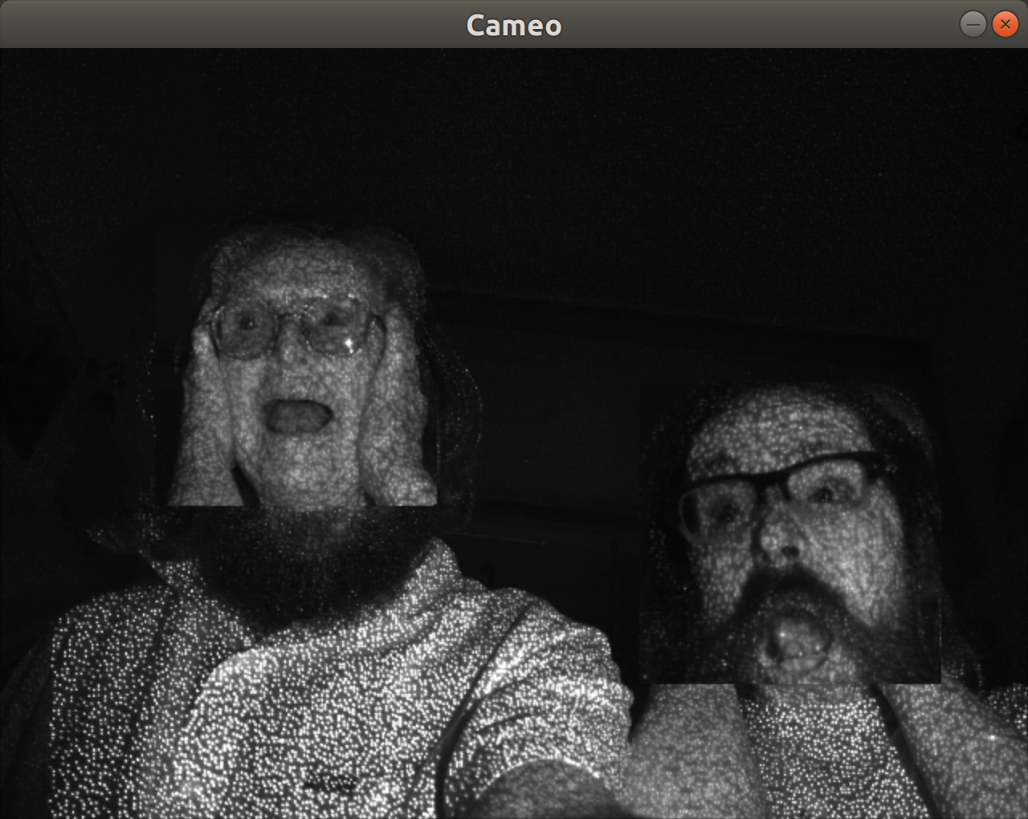
Here, we see the face of Joseph Howse swapped with the face of Janet Howse, his mother. Although Cameo is copying pixels from rectangular regions (and this is clearly visible at the bottom of the swapped regions, in the foreground), some of the background pixels within the rectangles are masked based on depth and thus are not swapped, so we do not see rectangular edges everywhere.You can find all of the relevant changes to the Cameo source code in this book's repository at https://github.com/PacktPublishing/Learning-OpenCV-5-Computer-Vision-with-Python-Fourth-Edition, specifically in the chapter05/cameo folder. For brevity, we will not discuss all of the changes here in this book, but we will cover some of the highlights in the next two subsections, Modifying the application's loop and Masking a copy operation.
Modifying the application's loop
To support face swapping, the Cameo project has two new modules called rects and trackers. The rects module contains functions for copying and swapping rectangles, with an optional mask to limit the copy or swap operation to particular pixels. The trackers module contains a class called FaceTracker, which adapts OpenCV's face detection functionality to an object-oriented style of programming.As we have covered OpenCV's face detection functionality earlier in this chapter, and we have demonstrated an object-oriented programming style in previous chapters, we will not go into the FaceTracker implementation here. Instead, you may look at it in this book's repository.Let's open cameo.py so that we can walk through the overall changes to the application:
- Near the top of the file, we need to import our new modules, as
highlightedhighlightedin the following code block:
import cv2
import depth
import filters
from managers import WindowManager, CaptureManager
import rects
from trackers import FaceTracker- Now, let's turn our attention to changes in the
__init__method of ourCameoDepthclass. Our updated application uses an instance ofFaceTracker. As part of its functionality,FaceTrackercan draw rectangles around detected faces. Let's give Cameo's user the option to enable or disable the drawing of face rectangles. We will keep track of the currently selected option via a Boolean variable. The following code blockhighlightsthe necessary changes to initialize theFaceTrackerobject and the Boolean variable:
class CameoDepth(Cameo):
    def __init__(self):
        self._windowManager = WindowManager('Cameo',
                                            self.onKeypress)
        #device = cv2.CAP_OPENNI2 # uncomment for Kinect
        device = cv2.CAP_OPENNI2_ASUS # uncomment for Xtion
        self._captureManager = CaptureManager(
            cv2.VideoCapture(device), self._windowManager, True)
        self._faceTracker = FaceTracker()
        self._shouldDrawDebugRects = False
        self._curveFilter = filters.BGRPortraCurveFilter()
We make use of the FaceTracker object in the run method of CameoDepth, which contains the application's main loop that captures and processes frames. Every time we successfully capture a frame, we call methods of FaceTracker to update the face detection result and get the latest detected faces. Then, for each face, we create a mask based on the depth camera's disparity map. (Previously, in Chapter 4, Depth Estimation and Segmentation, we created such a mask for the entire image instead of a mask for each face rectangle.)
- Then, we call a function,
rects.swapRects, to perform a masked swap of the face rectangles. (We will look at the implementation ofswapRectsa little later, in the Masking a copy operation section.) Depending on the currently selected option, we might tellFaceTrackerto draw rectangles around the faces. All of the relevant changes arehighlightedin the following code block:
    def run(self):
        """Run the main loop."""
        self._windowManager.createWindow()
        while self._windowManager.isWindowCreated:
            # ... The logic for capturing a frame is unchanged ...
            if frame is not None:
                self._faceTracker.update(frame)
                faces = self._faceTracker.faces
                masks = [
                    depth.createMedianMask(
                        disparityMap, validDepthMask,
                        face.faceRect)
                    for face in faces
                ]
                rects.swapRects(frame, frame,
                                [face.faceRect for face in faces],
                                masks)
                if self._captureManager.channel == cv2.CAP_OPENNI_BGR_IMAGE:
                    # A BGR frame was captured.
                    # Apply filters to it.
                    filters.strokeEdges(frame, frame)
                    self._curveFilter.apply(frame, frame)
                if self._shouldDrawDebugRects:
                    self._faceTracker.drawDebugRects(frame)
            self._captureManager.exitFrame()
self._windowManager.processEvents()- Finally, let's modify the
onKeypressmethod so that the user can hit the X key to start or stop displaying rectangles around detected faces. Again, the relevant changes arehighlightedin the following code block:
    def onKeypress(self, keycode):
        """Handle a keypress.
        space -> Take a screenshot.
        tab -> Start/stop recording a screencast.
        x -> Start/stop drawing debug rectangles around faces.
        escape -> Quit.
        """
        if keycode == 32: # space
            self._captureManager.writeImage('screenshot.png')
        elif keycode == 9: # tab
            if not self._captureManager.isWritingVideo:
                self._captureManager.startWritingVideo(
                    'screencast.avi')
            else:
                self._captureManager.stopWritingVideo()
        elif keycode == 120: # x
            self._shouldDrawDebugRects =
                not self._shouldDrawDebugRects
        elif keycode == 27: # escape
            self._windowManager.destroyWindow()
Next, let's look at the implementation of the rects module that we imported earlier in this section.
Masking a copy operation
The rects module is implemented in rects.py. We already saw a call to the rects.swapRects function in the previous section. However, before we consider the implementation of swapRects, we first need a more basic copyRect function.As far back as Chapter 2, Handling Files, Cameras, and GUIs, we learned how to copy data from one rectangular region of interest (ROI) to another using NumPy's slicing syntax. Outside the ROIs, the source and destination images were unaffected. Now, we want to apply further limits to this copy operation. We want to use a given mask that has the same dimensions as the source rectangle.We shall copy only those pixels in the source rectangle where the mask's value is not zero. Other pixels shall retain their old values from the destination image. This logic, with an array of conditions and two arrays of possible output values, can be expressed concisely with the numpy.where function.With this approach in mind, let's consider our copyRect function. As arguments, it takes a source and destination image, a source and destination rectangle, and a mask. The latter may be None, in which case, we simply resize the content of the source rectangle to match the destination rectangle and then assign the resulting resized content to the destination rectangle. Otherwise, we next ensure that the mask and the images have the same number of channels. We assume that the mask has one channel but the images may have three channels (BGR). We can add duplicate channels to mask using the repeat and reshape methods of numpy.array. Finally, we perform the copy operation using numpy.where. The complete implementation is as follows:
def copyRect(src, dst, srcRect, dstRect, mask = None,
             interpolation = cv2.INTER_LINEAR):
    """Copy part of the source to part of the destination."""
    x0, y0, w0, h0 = srcRect
    x1, y1, w1, h1 = dstRect
    # Resize the contents of the source sub-rectangle.
    # Put the result in the destination sub-rectangle.
    if mask is None:
        dst[y1:y1+h1, x1:x1+w1] =
            cv2.resize(src[y0:y0+h0, x0:x0+w0], (w1, h1),
                       interpolation = interpolation)
    else:
        if not utils.isGray(src):
            # Convert the mask to 3 channels, like the image.
            mask = mask.repeat(3).reshape(h0, w0, 3)
        # Perform the copy, with the mask applied.
        dst[y1:y1+h1, x1:x1+w1] =
            numpy.where(cv2.resize(mask, (w1, h1),
                                   interpolation =
                                   cv2.INTER_NEAREST),
                        cv2.resize(src[y0:y0+h0, x0:x0+w0], (w1, h1),
                                   interpolation = interpolation),
                        dst[y1:y1+h1, x1:x1+w1])
We also need to define a swapRects function, which uses copyRect to perform a circular swap of a list of rectangular regions. swapRects has a masks argument, which is a list of masks whose elements are passed to the respective copyRect calls. If the value of the masks argument is None, we pass None to every copyRect call. The following code shows the full implementation of swapRects:
def swapRects(src, dst, rects, masks = None,
              interpolation = cv2.INTER_LINEAR):
    """Copy the source with two or more sub-rectangles swapped."""
    if dst is not src:
        dst[:] = src
    numRects = len(rects)
    if numRects < 2:
        return
    if masks is None:
        masks = [None] * numRects
    # Copy the contents of the last rectangle into temporary storage.
    x, y, w, h = rects[numRects - 1]
    temp = src[y:y+h, x:x+w].copy()
    # Copy the contents of each rectangle into the next.
    i = numRects - 2
    while i >= 0:
        copyRect(src, dst, rects[i], rects[i+1], masks[i],
                 interpolation)
        i -= 1
    # Copy the temporarily stored content into the first rectangle.
    copyRect(temp, dst, (0, 0, w, h), rects[0], masks[numRects - 1],
             interpolation)
Note that the mask argument in copyRect and the masks argument in swapRects both have a default value of None. If no mask is specified, these functions copy or swap the entire contents of the rectangle or rectangles.
Summary
By now, you should have a good understanding of how face detection and face recognition work and how to implement them in Python and OpenCV 5.The accuracy of detection and recognition algorithms heavily depends on the quality of the training data, so make sure you provide your applications with a large number of training images covering a variety of expressions, poses, and lighting conditions. Later in this book, in Chapter 11, Neutral Networks with OpenCV – an Introduction, we will look at how to use several robust, pre-trained face detection models that build atop advanced algorithms and large sets of training data.As human beings, we might be predisposed to think that human faces are particularly recognizable. We might even be overconfident in our own face recognition abilities. However, in computer vision, there is nothing very special about human faces, and we can just as readily use algorithms to find and identify other things. We will begin to do so next in Chapter 6, Retrieving Images and Searching Using Image Descriptors.
Join our book community on Discord