
6 Retrieving Images and Searching Using Image Descriptors
Similar to the human eyes and brain, OpenCV can detect the main features of an image and extract them into so-called image descriptors. These features can then be used as a database, enabling image-based searches. Moreover, we can use key points to stitch images together and compose a bigger image. (Think of putting together many pictures to form a 360° panorama.)This chapter will show you how to detect the features of an image with OpenCV and make use of them to match and search images. Over the course of this chapter, we will take sample images and detect their main features, and then try to find a region of another image that matches the sample image. We will also find the homography or spatial relationship between a sample image and a matching region of another image.More specifically, we will cover the following tasks:
- Detecting keypoints and extracting local descriptors around the keypoints using any of the following algorithms: Harris corners, SIFT, SURF, or ORB
- Matching keypoints using brute-force algorithms or the FLANN algorithm
- Filtering out bad matches using KNN and the ratio test
- Finding the homography between two sets of matching keypoints
- Searching a set of images to determine which one contains the best match for a reference image
We will finish this chapter by building a proof-of-concept forensic application. Given a reference image of a tattoo, we will search for a set of images of people in order to find a person with a matching tattoo.
Technical requirements
This chapter uses Python, OpenCV, and NumPy. In regards to OpenCV, we use the optional opencv_contrib modules, which include additional algorithms for keypoint detection and matching. To enable theSURF algorithm (whichis patented and not free for commercial use), we must configure the opencv_contrib modules with the OPENCV_ENABLE_NONFREE flag in CMake. Please refer to Chapter 1, Setting Up OpenCV, for installation instructions. Additionally, if you have not already installed Matplotlib, install it by running $ pip install matplotlib (or $ pip3 install matplotlib, depending on your environment).The complete code for this chapter can be found in this book's GitHub repository, https://github.com/PacktPublishing/Learning-OpenCV-5-Computer-Vision-with-Python-Fourth-Edition, in the chapter06 folder. The sample images can be found in the images folder.A subset of the chapter’s sample code can be edited and run interactively in Google Colab at https://colab.research.google.com/github/PacktPublishing/Learning-OpenCV-5-Computer-Vision-with-Python-Fourth-Edition/blob/main/chapter06/chapter06.ipynb.
Understanding types of feature detection and matching
A number of algorithms can be used to detect and describe features, and we will explore several of them in this section. The most commonly used feature detection and descriptor extraction algorithms in OpenCV are as follows:
- Harris: This algorithm is useful for detecting corners.
- SIFT: This algorithm is useful for detecting blobs.
- SURF: This algorithm is useful for detecting blobs.
- FAST: This algorithm is useful for detecting corners.
- BRIEF: This algorithm is useful for detecting blobs.
- ORB: This algorithm stands for Oriented FAST and Rotated BRIEF. It is useful for detecting a combination of corners and blobs.
Matching features can be performed with the following methods:
- Brute-force matching
- FLANN-based matching
Spatial verification can then be performed with homography.We have just introduced a lot of new terminology and algorithms. Now, we will go over their basic definitions.
Defining features
What is a feature, exactly? Why is a particular area of an image classifiable as a feature, while others are not? Broadly speaking, a feature is an area of interest in the image that is unique or easily recognizable. Corners and regions with a high density of textural detail are good features, while patterns that repeat themselves a lot and low-density regions (such as a blue sky) are not. Edges are good features as they tend to divide two regions with abrupt changes in the intensity (gray or color) values of an image. A blob (a region of an image that greatly differs from its surrounding areas) is also an interesting feature.Most feature detection algorithms revolve around the identification of corners, edges, and blobs, with some also focusing on the concept of a ridge, which you can conceptualize as the axis of symmetry of an elongated object. (Think, for example, about identifying a road in an image.)Some algorithms are better at identifying and extracting features of a certain type, so it is important to know what your input image is so that you can utilize the best tool in your OpenCV belt.
Detecting Harris corners
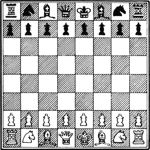
Let's start by finding corners using the Harris corner detection algorithm. We will do this by implementing an example. If you continue to study OpenCV beyond this book, you will find that chessboards are a common subject of analysis in computer vision, partly because a checkered pattern is suited to many types of feature detection, and partly because chess is a popular pastime, especially in Russia, which is the country of origin of many of OpenCV's developers.Here is our sample image of a chessboard and chess pieces:
OpenCV has a handy function called cv2.cornerHarris, which detects corners in an image. We can see this function at work in the following basic example:
import cv2
img = cv2.imread('../images/chess_board.png')
gray = cv2.cvtColor(img, cv2.COLOR_BGR2GRAY)
dst = cv2.cornerHarris(gray, 2, 23, 0.04)
img[dst > 0.01 * dst.max()] = [0, 0, 255]
cv2.imshow('corners', img)
cv2.waitKey()
Let's analyze the code. After the usual imports, we load the chessboard image and convert it into grayscale. Then, we call the cornerHarris function:
dst = cv2.cornerHarris(gray, 2, 23, 0.04)The most important parameter here is the third one, which defines the aperture or kernel size of the Sobel operator. The Sobel operator detects edges by measuring horizontal and vertical differences between pixel values in a neighborhood, and it does this using a kernel. The cv2.cornerHarris function uses a Sobel operator whose aperture is defined by this parameter. In plain English, the parameters define how sensitive corner detection is. It must be between 3 and 31 and be an odd value. With a low (highly sensitive) value of 3, all those diagonal lines in the black squares of the chessboard will register as corners when they touch the border of the square. For a higher (less sensitive) value of 23, only the corners of each square will be detected as corners.cv2.cornerHarris returns an image in floating-point format. Each value in this image represents a score for the corresponding pixel in the source image. A moderate or high score indicates that the pixel is likely to be a corner. Conversely, we can treat pixels with the lowest scores as non-corners. Consider the following line:
img[dst > 0.01 * dst.max()] = [0, 0, 255]Here, we select pixels with scores that are at least 1% of the highest score, and we color these pixels red in the original image. Here is the result:
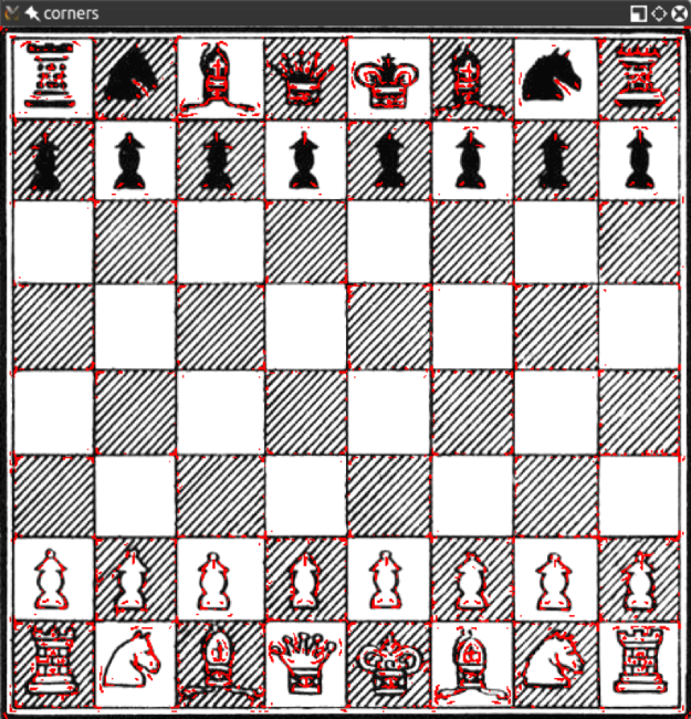
Great! Nearly all the detected corners are marked in red. The marked points include nearly all the corners of the chessboard's squares.
If we tweak the second parameter in
cv2.cornerHarris, we will see that smaller regions (for a smaller parameter value) or larger regions (for a larger parameter value) will be detected as corners. This parameter is called the block size.
Detecting DoG features and extracting SIFT descriptors
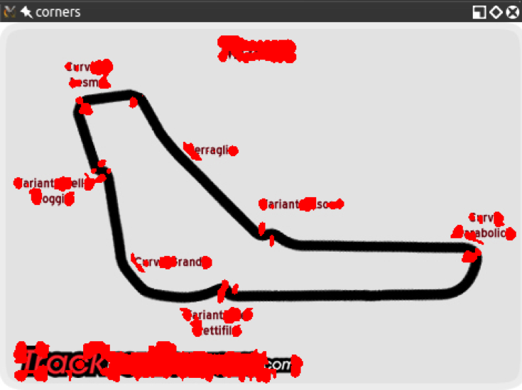
The preceding technique, which uses cv2.cornerHarris, is great for detecting corners and has a distinct advantage because even if the image is rotated corners are still the corners. However, if we scale an image to a smaller or larger size, some parts of the image may lose or even gain a corner quality.For example, take a look at the following corner detections in an image of the F1 Italian Grand Prix track:
Here is the corner detection result with a smaller version of the same image:
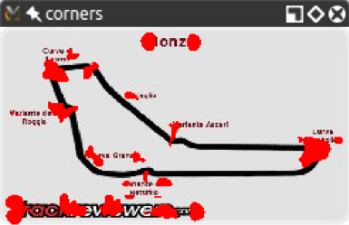
You will notice how the corners are a lot more condensed; however, even though we gained some corners, we lost others! In particular, let's examine the Variante Ascari chicane, which looks like a squiggle at the end of the part of the track that runs straight from northwest to southeast. In the larger version of the image, both the entrance and the apex of the double bend were detected as corners. In the smaller image, the apex is not detected as such. If we further reduce the image, at some scale, we will lose the entrance to that chicane too.This loss of features raises an issue; we need an algorithm that works regardless of the scale of the image. Enter Scale-Invariant Feature Transform (SIFT). While the name may sound a bit mysterious, now that we know what problem we are trying to solve, it actually makes sense. We need a function (a transform) that will detect features (a feature transform) and will not output different results depending on the scale of the image (a scale-invariant feature transform). Note that SIFT does not detect keypoints. Keypoint detection is done with the Difference of Gaussians (DoG), while SIFT describes the region surrounding the keypoints by means of a feature vector.A quick introduction to the DoG is in order. Previously, in Chapter 3, Processing Images with OpenCV, we talked about low pass filters and blurring operations, and specifically the cv2.GaussianBlur function. DoG is the result of applying different Gaussian filters to the same image. Previously, we applied this type of technique for edge detection, and the idea is the same here. The final result of a DoG operation contains areas of interest (keypoints), which are then going to be described through SIFT.Let's see how DoG and SIFT behave in the following image, which is full of corners and features:
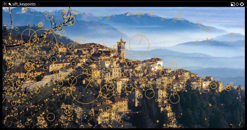
Here, the beautiful panorama of Varese (in Lombardy, Italy) gains a new type of fame as a subject of computer vision. Here is the code that produces this processed image:
import cv2
img = cv2.imread('../images/varese.jpg')
gray = cv2.cvtColor(img, cv2.COLOR_BGR2GRAY)
sift = cv2.SIFT_create()
keypoints, descriptors = sift.detectAndCompute(gray, None)
cv2.drawKeypoints(img, keypoints, img, (51, 163, 236),
                  cv2.DRAW_MATCHES_FLAGS_DRAW_RICH_KEYPOINTS)
cv2.imshow('sift_keypoints', img)
cv2.waitKey()
After the usual imports, we load the image we want to process. Then, we convert the image into grayscale. By now, you may have gathered that many methods in OpenCV expect a grayscale image as input. The next step is to create a SIFT detection object and compute the features and descriptors of the grayscale image:
sift = cv2.SIFT_create()
keypoints, descriptors = sift.detectAndCompute(gray, None)
Behind the scenes, these simple lines of code carry out an elaborate process; we create a cv2.SIFT object, which uses DoG to detect keypoints and then computes a feature vector for the surrounding region of each keypoint. As the name of the detectAndCompute method clearly suggests, two main operations are performed: feature detection and the computation of descriptors. The return value of the operation is a tuple containing a list of keypoints and another list of the keypoints' descriptors.Finally, we process this image by drawing the keypoints on it with the cv2.drawKeypoints function and then displaying it with the usual cv2.imshow function. As one of its arguments, the cv2.drawKeypoints function accepts a flag that specifies the type of visualization we want. Here, we specify cv2.DRAW_MATCHES_FLAGS_DRAW_RICH_KEYPOINT in order to draw a visualization of the scale and orientation of each keypoint.
Anatomy of a keypoint
Each keypoint is an instance of the cv2.KeyPoint class, which has the following properties:
- The
pt(point) property contains the x and y coordinates of the keypoint in the image. - The
sizeproperty indicates the diameter of the feature. - The
angleproperty indicates the orientation of the feature, as shown by the radial lines in the preceding processed image. - The
responseproperty indicates the strength of the keypoint. Some features are classified by SIFT as stronger than others, andresponseis the property you would check to evaluate the strength of a feature. - The
octaveproperty indicates the layer in the image pyramid where the feature was found. Let's briefly review the concept of an image pyramid, which we discussed previously in Chapter 5, Detecting and Recognizing Faces, in the Conceptualizing Haar cascades section. The SIFT algorithm operates in a similar fashion to face detection algorithms in that it processes the same image iteratively but alters the input at each iteration. In particular, the scale of the image is a parameter that changes at each iteration (octave) of the algorithm. Thus, theoctaveproperty is related to the image scale at which the keypoint was detected. - Finally, the
class_idproperty can be used to assign a custom identifier to a keypoint or a group of keypoints.
Detecting Fast Hessian features and extracting SURF descriptors
Computer vision is a relatively young branch of computer science, so many famous algorithms and techniques have only been invented recently. SIFT is, in fact, only 23 years old, having been published by David Lowe in 1999.SURF is a feature detection algorithm that was published in 2006 by Herbert Bay. SURF is several times faster than SIFT, and it is partially inspired by it.
Note that SURF is a patented algorithm and, for this reason, is made available only in builds of
opencv_contribwhere theOPENCV_ENABLE_NONFREECMake flag is used. SIFT was formerly a patented algorithm but its patent expired and now SIFT is available in standard builds of OpenCV.
It is not particularly relevant to this book to understand how SURF works under the hood, inasmuch as we can use it in our applications and make the best of it. What is important to understand is that cv2.SURF is an OpenCV class that performs keypoint detection with the Fast Hessian algorithm and descriptor extraction with SURF, much like the cv2.SIFT class performs keypoint detection with DoG and descriptor extraction with SIFT.Also, the good news is that OpenCV provides a standardized API for all its supported feature detection and descriptor extraction algorithms. Thus, with only trivial changes, we can adapt our previous code sample to use SURF instead of SIFT. Here is the modified code, with the changes highlighted:
import cv2
img = cv2.imread('../images/varese.jpg')
gray = cv2.cvtColor(img, cv2.COLOR_BGR2GRAY)
surf = cv2.xfeatures2d.SURF_create(8000)
keypoints, descriptor = surf.detectAndCompute(gray, None)
cv2.drawKeypoints(img, keypoints, img, (51, 163, 236),
cv2.DRAW_MATCHES_FLAGS_DRAW_RICH_KEYPOINTS)
cv2.imshow('surf_keypoints', img)
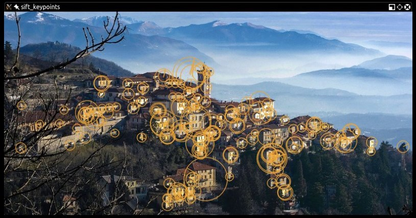
cv2.waitKey()The parameter to cv2.xfeatures2d.SURF_create is a threshold for the Fast Hessian algorithm. By increasing the threshold, we can reduce the number of features that will be retained. With a threshold of 8000, we get the following result:
Try adjusting the threshold to see how it affects the result. As an exercise, you may want to build a GUI application with a slider that controls the value of the threshold. This way, a user can adjust the threshold and see the number of features increase and decrease in an inversely proportional fashion. We built a GUI application with sliders in Chapter 4, Depth Estimation and Segmentation, in the Depth estimation with a normal camera section, so you may want to refer back to that section as a guide.Next, we'll examine the FAST corner detector, the BRIEF keypoint descriptor, and ORB (which uses FAST and BRIEF together).
Using ORB with FAST features and BRIEF descriptors
If SIFT is young, and SURF younger, ORB is in its infancy. ORB was first published in 2011 as a fast alternative to SIFT and SURF.The algorithm was published in the paper ORB: an efficient alternative to SIFT or SURF, available in PDF format at http://www.willowgarage.com/sites/default/files/orb_final.pdf.ORB mixes the techniques used in the FAST keypoint detector and the BRIEF keypoint descriptor, so it is worth taking a quick look at FAST and BRIEF first. Then, we will talk about brute-force matching – an algorithm used for feature matching – and look at an example of feature matching.
FAST
The Features from Accelerated Segment Test (FAST) algorithm works by analyzing circular neighborhoods of 16 pixels. It marks each pixel in a neighborhood as brighter or darker than a particular threshold, which is defined relative to the center of the circle. A neighborhood is deemed to be a corner if it contains a number of contiguous pixels marked as brighter or darker.FAST also uses a high-speed test, which can sometimes determine that a neighborhood is not a corner by checking just 2 or 4 pixels instead of 16. To understand how this test works, let's take a look at the following diagram, taken from the OpenCV documentation:
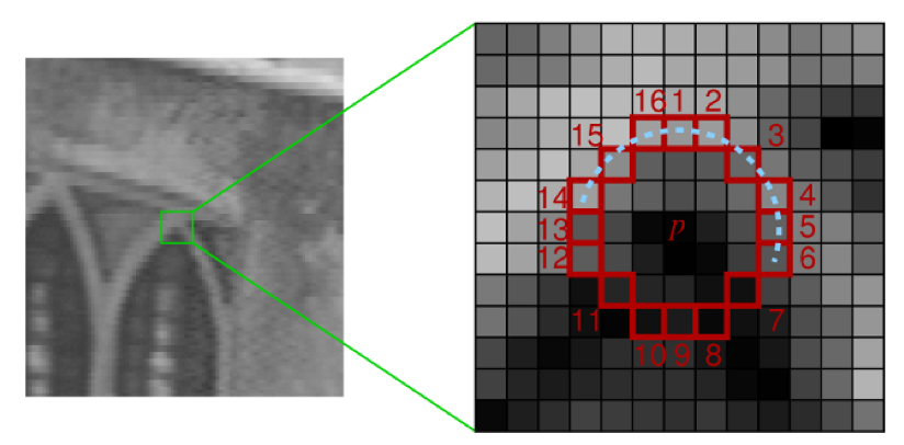
Here, we can see a 16-pixel neighborhood at two different magnifications. The pixels at positions 1, 5, 9, and 13 correspond to the four cardinal points at the edge of the circular neighborhood. If the neighborhood is a corner, we expect that out of these four pixels, exactly three or exactly one will be brighter than the threshold. (Another way of saying this is that exactly one or exactly three of them will be darker than the threshold.) If exactly two of them are brighter than the threshold, then we have an edge, not a corner. If exactly four or exactly zero of them are brighter than the threshold, then we have a relatively uniform neighborhood that is neither a corner nor an edge.FAST is a clever algorithm, but it's not devoid of weaknesses, and to compensate for these weaknesses, developers analyzing images can implement a machine learning approach in order to feed a set of images (relevant to a given application) to the algorithm so that parameters such as the threshold are optimized. Whether the developer specifies parameters directly or provides a training set for a machine learning approach, FAST is an algorithm that is sensitive to the developer's input, perhaps more so than SIFT.
BRIEF
Binary Robust Independent Elementary Features (BRIEF), on the other hand, is not a feature detection algorithm, but a descriptor. Let's delve deeper into the concept of what a descriptor is, and then look at BRIEF.When we previously analyzed images with SIFT and SURF, the heart of the entire process was the call to the detectAndCompute function. This function performs two different steps – detection and computation – and they return two different results, coupled in a tuple.The result of detection is a set of keypoints; the result of the computation is a set of descriptors for those keypoints. This means that OpenCV's cv2.SIFT and cv2.xfeatures2d.SURF classes implement algorithms for both detection and description. Remember, though, that the original SIFT and SURF are not feature detection algorithms. OpenCV's cv2.SIFT implements DoG feature detection plus SIFT description, while OpenCV's cv2.xfeatures2d.SURF implements Fast Hessian feature detection plus SURF description.Keypoint descriptors are a representation of the image that serves as the gateway to feature matching because you can compare the keypoint descriptors of two images and find commonalities.BRIEF is one of the fastest descriptors currently available. The theory behind BRIEF is quite complicated, but suffice it to say that BRIEF adopts a series of optimizations that make it a very good choice for feature matching.
Brute-force matching
A brute-force matcher is a descriptor matcher that compares two sets of keypoint descriptors and generates a result that is a list of matches. It is called brute-force because little optimization is involved in the algorithm. For each keypoint descriptor in the first set, the matcher makes comparisons to every keypoint descriptor in the second set. Each comparison produces a distance value and the best match can be chosen on the basis of least distance.More generally, in computing, the term brute-force is associated with an approach that prioritizes the exhaustion of all possible combinations (for example, all the possible combinations of characters to crack a password of a known length). Conversely, an algorithm that prioritizes speed might skip some possibilities and try to take a shortcut to the solution that seems the most plausible.OpenCV provides a cv2.BFMatcher class that supports several approaches to brute-force feature matching.
Matching a logo in two images
Now that we have a general idea of what FAST and BRIEF are, we can understand why the team behind ORB (composed of Ethan Rublee, Vincent Rabaud, Kurt Konolige, and Gary R. Bradski) chose these two algorithms as a foundation for ORB.In their paper, the authors set out to achieve the following results:
- The addition of a fast and accurate orientation component to FAST
- The efficient computation of oriented BRIEF features
- Analysis of variance and correlation of oriented BRIEF features
- A learning method to decorrelate BRIEF features under rotational invariance, leading to better performance in nearest-neighbor applications
The main points are quite clear: ORB aims to optimize and speed up operations, including the very important step of utilizing BRIEF in a rotation-aware fashion so that matching is improved, even in situations where a training image has a very different rotation to the query image.At this stage, though, perhaps you have had enough of the theory and want to sink your teeth into some feature matching, so let's look at some code. The following script attempts to match features in a logo to the features in a photograph that contains the logo:
import cv2
from matplotlib import pyplot as plt
# Load the images.
img0 = cv2.imread('../images/nasa_logo.png',
                  cv2.IMREAD_GRAYSCALE)
img1 = cv2.imread('../images/kennedy_space_center.jpg',
                  cv2.IMREAD_GRAYSCALE)
# Perform ORB feature detection and description.
orb = cv2.ORB_create()
kp0, des0 = orb.detectAndCompute(img0, None)
kp1, des1 = orb.detectAndCompute(img1, None)
# Perform brute-force matching.
bf = cv2.BFMatcher(cv2.NORM_HAMMING, crossCheck=True)
matches = bf.match(des0, des1)
# Sort the matches by distance.
matches = sorted(matches, key=lambda x:x.distance)
# Draw the best 25 matches.
img_matches = cv2.drawMatches(
    img0, kp0, img1, kp1, matches[:25], img1,
    flags=cv2.DRAW_MATCHES_FLAGS_NOT_DRAW_SINGLE_POINTS)
# Show the matches.
plt.imshow(img_matches)
plt.show()
Let's examine this code step by step. After the usual imports, we load two images (the query image and the scene) in grayscale format. Here is the query image, which is the NASA logo:

Here is the photo of the scene, which is the Kennedy Space Center:

Now, we proceed to create the ORB feature detector and descriptor:
# Perform ORB feature detection and description.
orb = cv2.ORB_create()
kp0, des0 = orb.detectAndCompute(img0, None)
kp1, des1 = orb.detectAndCompute(img1, None)
In a similar fashion to what we did with SIFT and SURF, we detect and compute the keypoints and descriptors for both images.From here, the concept is pretty simple: iterate through the descriptors and determine whether they are a match or not, and then calculate the quality of this match (distance) and sort the matches so that we can display the top n matches with a degree of confidence that they are, in fact, matching features on both images. cv2.BFMatcher does this for us:
# Perform brute-force matching.
bf = cv2.BFMatcher(cv2.NORM_HAMMING, crossCheck=True)
matches = bf.match(des0, des1)
# Sort the matches by distance.
matches = sorted(matches, key=lambda x:x.distance)
At this stage, we already have all the information we need, but as computer vision enthusiasts, we place quite a bit of importance on visually representing data, so let's draw these matches in a matplotlib chart:
# Draw the best 25 matches.
img_matches = cv2.drawMatches(
    img0, kp0, img1, kp1, matches[:25], img1,
    flags=cv2.DRAW_MATCHES_FLAGS_NOT_DRAW_SINGLE_POINTS)
# Show the matches.
plt.imshow(img_matches)
plt.show()
Python's slicing syntax is quite robust. If the
matcheslist contains fewer than 25 entries, thematches[:25]slicing command will run without problems and give us a list with just as many elements as the original.
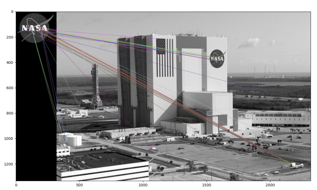
The result is as follows:
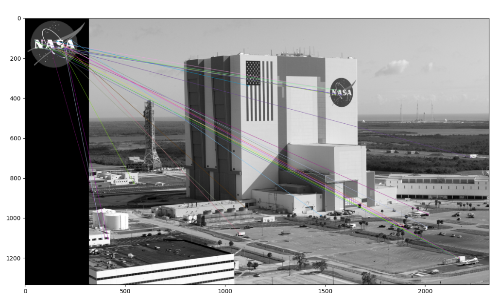
You might think that this is a disappointing result. Indeed, we can see that most of the matches are false matches. Unfortunately, this is quite typical. To improve our results, we need to apply additional techniques to filter out bad matches. We'll turn our attention to this task next.
Filtering matches using K-Nearest Neighbors and the ratio test
Imagine that a large group of renowned philosophers asks you to judge their debate on a question of great importance to life, the universe, and everything. You listen carefully as each philosopher speaks in turn. Finally, when all the philosophers have exhausted all their lines of argument, you review your notes and perceive two things, as follows:
- Every philosopher disagrees with every other
- No one philosopher is much more convincing than the others
From your first observation, you infer that at most one of the philosophers is right; however, it is possible that all the philosophers could be wrong. Then, from your second observation, you begin to fear that you are at risk of picking a philosopher who is wrong, even if one of the philosophers is correct. Any way you look at it, these people have made you late for dinner. You call it a tie and say that the debate's all-important question remains unresolved.We can compare our imaginary problem of judging the philosophers' debate to our practical problem of filtering out bad keypoint matches.First, let's assume that each keypoint in our query image has, at most, one correct match in the scene. By implication, if our query image is the NASA logo, we assume that the other image – the scene – contains, at most, one NASA logo. Given that a query keypoint has, at most, one correct or good match, when we consider all possible matches, we are primarily observing bad matches. Thus, a brute-force matcher, which computes a distance score for every possible match, can give us plenty of observations of the distance scores for bad matches. We expect that a good match will have a significantly better (lower) distance score than the numerous bad matches, so the scores for the bad matches can help us pick a threshold for a good match. Such a threshold does not necessarily generalize well across different query keypoints or different scenes, but at least it helps us on a case-by-case basis.Now, let's consider the implementation of a modified brute-force matching algorithm that adaptively chooses a distance threshold in the manner we have described. In the previous section's code sample, we used the match method of the cv2.BFMatcher class in order to get a list containing the single best (least-distance) match for each query keypoint. By doing so, we discarded information about the distance scores of all the worse possible matches – the kind of information we need for our adaptive approach. Fortunately, cv2.BFMatcher also provides a knnMatch method, which accepts an argument, k, that specifies the maximum number of best (least-distance) matches that we want to retain for each query keypoint. (In some cases, we may get fewer matches than the maximum.) KNN stands for k-nearest neighbors.We will use the knnMatch method to request a list of the two best matches for each query keypoint. Based on our assumption that each query keypoint has, at most, one correct match, we are confident that the second-best match is wrong. We multiply the second-best match's distance score by a value less than 1 in order to obtain the threshold.Then, we accept the best match as a good match only if its distant score is less than the threshold. This approach is known as the ratio test, and it was first proposed by David Lowe, the author of the SIFT algorithm. He describes the ratio test in his paper, Distinctive Image Features from Scale-Invariant Keypoints, which is available at https://www.cs.ubc.ca/~lowe/papers/ijcv04.pdf. Specifically, in the Application to object recognition section, he states the following:
"The probability that a match is correct can be determined by taking the ratio of the distance from the closest neighbor to the distance of the second closest."
We can load the images, detect keypoints, and compute ORB descriptors in the same way as we did in the previous section's code sample. Then, we can perform brute-force KNN matching using the following two lines of code:
# Perform brute-force KNN matching.
bf = cv2.BFMatcher(cv2.NORM_HAMMING, crossCheck=False)
pairs_of_matches = bf.knnMatch(des0, des1, k=2)
knnMatch returns a list of lists; each inner list contains at least one match and no more than k matches, sorted from best (least distance) to worst. The following line of code sorts the outer list based on the distance score of the best matches:
# Sort the pairs of matches by distance.
pairs_of_matches = sorted(pairs_of_matches, key=lambda x:x[0].distance)
Let's draw the top 25 best matches, along with any second-best matches that knnMatch may have paired with them. We can't use the cv2.drawMatches function because it only accepts a one-dimensional list of matches; instead, we must use cv2.drawMatchesKnn. The following code is used to select, draw, and show the matches:
# Draw the 25 best pairs of matches.
img_pairs_of_matches = cv2.drawMatchesKnn(
    img0, kp0, img1, kp1, pairs_of_matches[:25], img1,
    flags=cv2.DRAW_MATCHES_FLAGS_NOT_DRAW_SINGLE_POINTS)
# Show the pairs of matches.
plt.imshow(img_pairs_of_matches)
plt.show()
So far, we have not filtered out any bad matches – and, indeed, we have deliberately included the second-best matches, which we believe to be bad – so the result looks a mess. Here it is:
Now, let's apply the ratio test. We will set the threshold at 0.8 times the distance score of the second-best match. If knnMatch has failed to provide a second-best match, we reject the best match anyway because we are unable to apply the test. The following code applies these conditions and provides us with a list of best matches that passed the test:
# Apply the ratio test.
matches = [x[0] for x in pairs_of_matches
           if len(x) > 1 and x[0].distance < 0.8 * x[1].distance]
Having applied the ratio test, now we are only dealing with best matches (not pairs of best and second-best matches), so we can draw them with cv2.drawMatches instead of cv2.drawMatchesKnn. Again, we will select the top 25 matches from the list. The following code is used to select, draw, and show the matches:
# Draw the best 25 matches.
img_matches = cv2.drawMatches(
    img0, kp0, img1, kp1, matches[:25], img1,
    flags=cv2.DRAW_MATCHES_FLAGS_NOT_DRAW_SINGLE_POINTS)
# Show the matches.
plt.imshow(img_matches)
plt.show()
Here, we can see the matches that passed the ratio test:
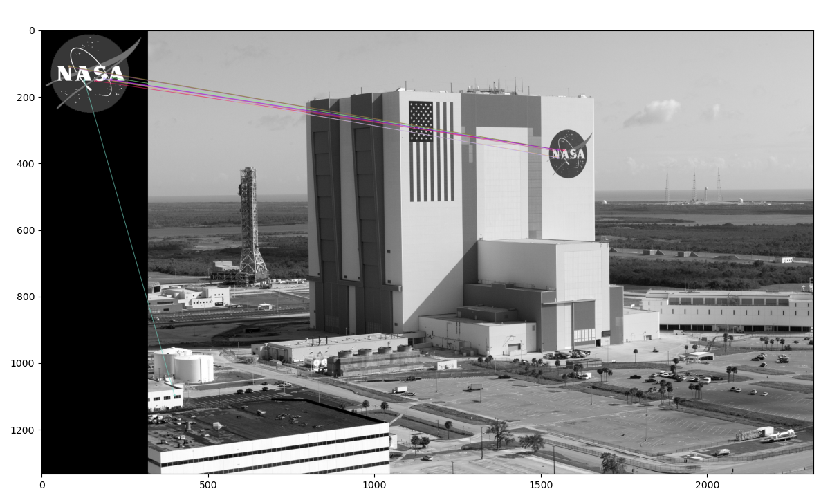
Comparing this output image to the one in the previous section, we can see that KNN and the ratio test have allowed us to filter out many bad matches. The remaining matches are not perfect but nearly all of them point to the correct region – the NASA logo on the side of the Kennedy Space Center.We have made a promising start. Next, we will replace the brute-force matcher with a faster matcher called FLANN. After that, we will learn how to describe a set of matches in terms of homography – that is, a 2D transformation matrix that expresses the position, rotation, scale, and other geometric characteristics of the matched object.
Matching with FLANN
FLANN stands for Fast Library for Approximate Nearest Neighbors. It is an open source library under the permissive 2-clause BSD license and it is available on GitHub at https://github.com/flann-lib/flann. There, we find the following description:
"FLANN is a library for performing fast approximate nearest neighbor searches in high dimensional spaces. It contains a collection of algorithms we found to work best for the nearest neighbor search and a system for automatically choosing the best algorithm and optimum parameters depending on the dataset. FLANN is written in C++ and contains bindings for the following languages: C, MATLAB,Python, and Ruby."
In other words, FLANN has a big toolbox, it knows how to choose the right tools for the job, and it speaks several languages. These features make the library fast and convenient. Indeed, FLANN's authors claim that it is 10 times faster than other nearest-neighbor search software for many datasets.Although FLANN is also available as a standalone library, we will use it as part of OpenCV because OpenCV provides a handy wrapper for it.To begin our practical example of FLANN matching, let's import NumPy, OpenCV, and Matplotlib, and load two images from files. Here is the relevant code:
import numpy as np
import cv2
from matplotlib import pyplot as plt
img0 = cv2.imread('../images/gauguin_entre_les_lys.jpg',
                  cv2.IMREAD_GRAYSCALE)
img1 = cv2.imread('../images/gauguin_paintings.png',
                  cv2.IMREAD_GRAYSCALE)
Here is the first image – the query image – that our script is loading:
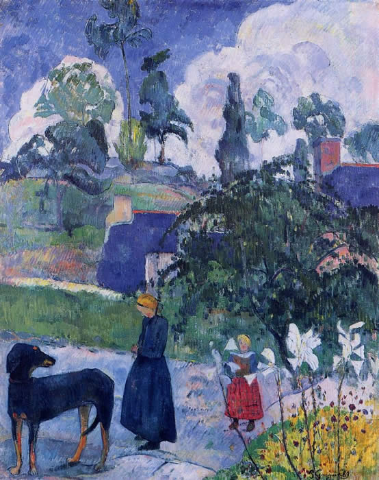
This work of art is Entre les lys (Among the lilies), painted by Paul Gauguin in 1889. We will search for matching keypoints in a larger image that contains multiple works by Gauguin, alongside some haphazard shapes drawn by one of the authors of this book. Here is the larger image:
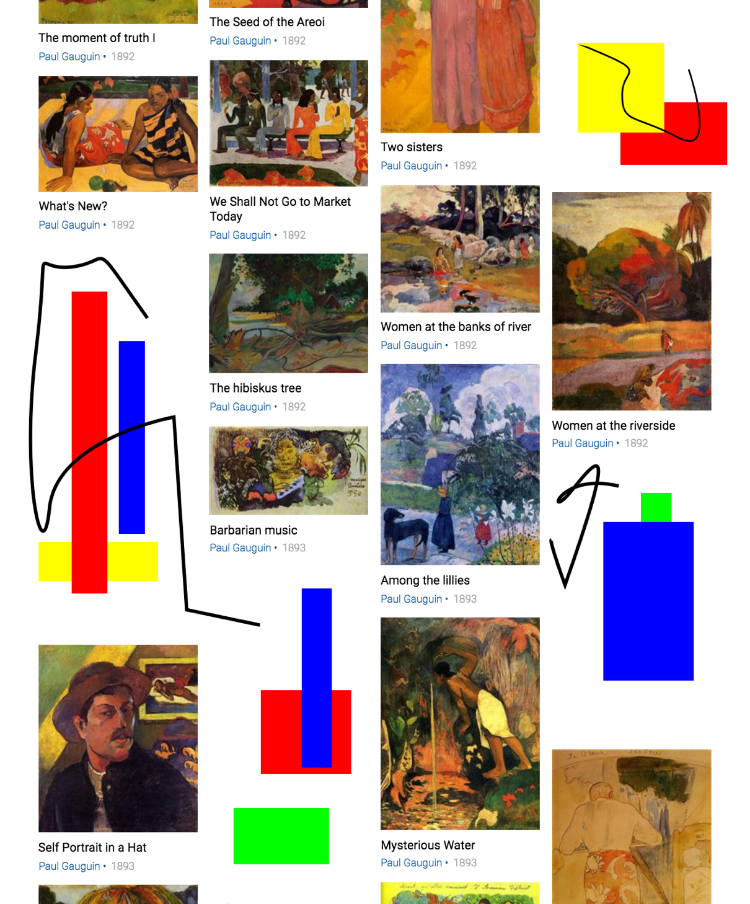
Within the larger image, Entre les lys appears in the third column, third row. The query image and the corresponding region of the larger image are not identical; they depict Entre les lys in slightly different colors and at a different scale. Nonetheless, this should be an easy case for our matcher.Let's detect the necessary keypoints and extract our features using the cv2.SIFT class:
# Perform SIFT feature detection and description.
sift = cv2.SIFT_create()
kp0, des0 = sift.detectAndCompute(img0, None)
kp1, des1 = sift.detectAndCompute(img1, None)
So far, the code should seem familiar, since we have already dedicated several sections of this chapter to SIFT and other descriptors. In our previous examples, we fed the descriptors to cv2.BFMatcher for brute-force matching. This time, we will use cv2.FlannBasedMatcher instead. The following code performs FLANN-based matching with custom parameters:
# Define FLANN-based matching parameters.
FLANN_INDEX_KDTREE = 1
index_params = dict(algorithm=FLANN_INDEX_KDTREE, trees=5)
search_params = dict(checks=50)
# Perform FLANN-based matching.
flann = cv2.FlannBasedMatcher(index_params, search_params)
matches = flann.knnMatch(des0, des1, k=2)
Here, we can see that the FLANN matcher takes two parameters: an indexParams object and a searchParams object. These parameters, passed in the form of dictionaries in Python (and structs in C++), determine the behavior of the index and search objects that are used internally by FLANN to compute the matches. We have chosen parameters that offer a reasonable balance between accuracy and processing speed. Specifically, we are using a kernel density tree (kd-tree) indexing algorithm with five trees, which FLANN can process in parallel. (The FLANN documentation recommends between one tree, which would offer no parallelism, and 16 trees, which would offer a high degree of parallelism if the system could exploit it.)We are performing 50 checks or traversals of each tree. A greater number of checks can provide greater accuracy but at a greater computational cost.After performing FLANN-based matching, we apply Lowe's ratio test with a multiplier of 0.7. To demonstrate a different coding style, we will use the result of the ratio test in a slightly different way compared to how we did in the previous section's code sample. Previously, we assembled a new list with just the good matches in it. This time, we will assemble a list called mask_matches, in which each element is a sublist of length k (the same k that we passed to knnMatch). If a match is good, we set the corresponding element of the sublist to 1; otherwise, we set it to 0.For example, if we have mask_matches = [[0, 0], [1, 0]], this means that we have two matched keypoints; for the first keypoint, the best and second-best matches are both bad, while for the second keypoint, the best match is good but the second-best match is bad. Remember, we assume that all the second-best matches are bad. We use the following code to apply the ratio test and build the mask:
# Prepare an empty mask to draw good matches.
mask_matches = [[0, 0] for i in range(len(matches))]
# Populate the mask based on David G. Lowe's ratio test.
for i, (m, n) in enumerate(matches):
    if m.distance < 0.7 * n.distance:
        mask_matches[i]=[1, 0]
Now, it is time to draw and show the good matches. We can pass our mask_matches list to cv2.drawMatchesKnn as an optional argument, as highlighted in the following code segment:
# Draw the matches that passed the ratio test.
img_matches = cv2.drawMatchesKnn(
    img0, kp0, img1, kp1, matches, None,
    matchColor=(0, 255, 0), singlePointColor=(255, 0, 0),
    matchesMask=mask_matches, flags=0)
# Show the matches.
plt.imshow(img_matches)
plt.show()
cv2.drawMatchesKnn only draws the matches that we marked as good (with a value of 1) in our mask. Let's unveil the result. Our script produces the following visualization of the FLANN-based matches:
This is an encouraging picture: it appears that nearly all the matches fall in the right places. Next, let's try to reduce this type of result to a more succinct geometric representation – a homography – which would describe the pose of a whole matched object rather than a bunch of disconnected matched points.
Finding homography with FLANN-based matches
First of all, what is homography? Let's read a definition from the internet:
"A relation between two figures, such that to any point of the one corresponds one and but one point in the other, and vice versa. Thus, a tangent line rolling on a circle cuts two fixed tangents of the circle in two sets of points that are homographic."
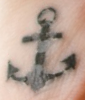
If you – like the authors of this book – are none the wiser from the preceding definition, you will probably find the following explanation a bit clearer: homography is a condition in which two figures find each other when one is a perspective distortion of the other.First, let's take a look at what we want to achieve so that we can fully understand what homography is. Then, we will go through the code.Imagine that we want to search for the following tattoo:
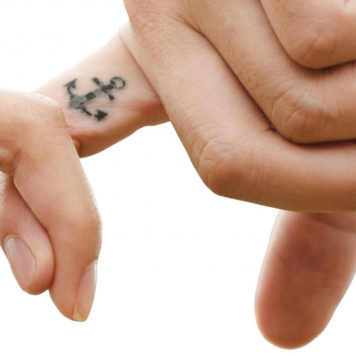
We, as human beings, can easily locate the tattoo in the following image, despite there being a difference in rotation:
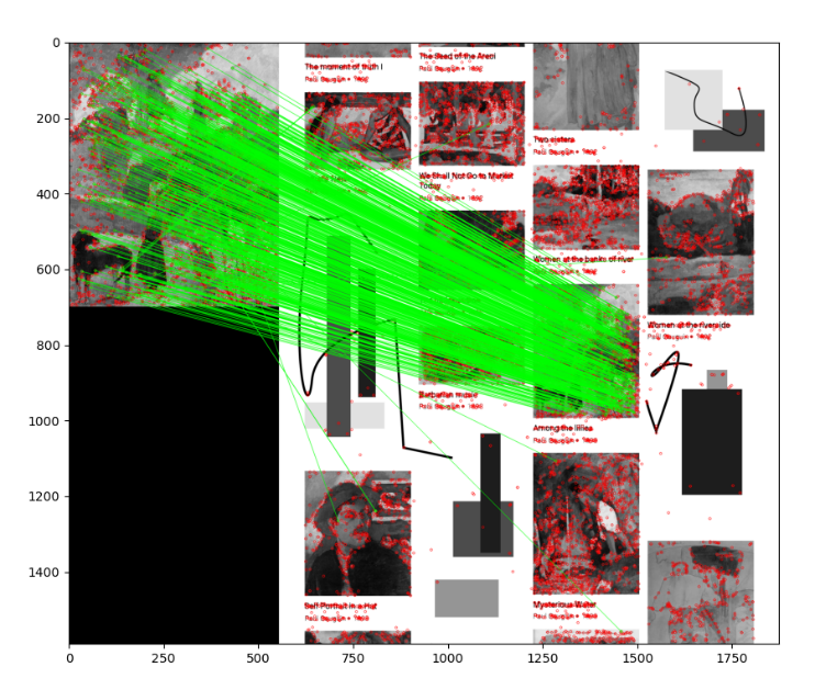
As an exercise in computer vision, we want to write a script that produces the following visualization of keypoint matches and the homography:
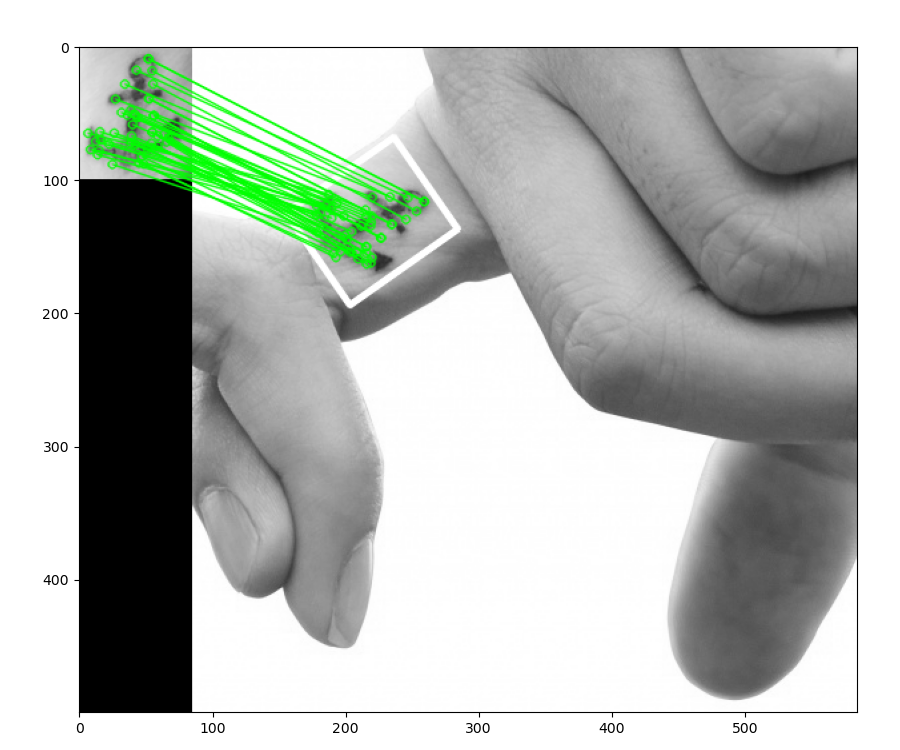
As shown in the preceding screenshot, we took the subject in the first image, correctly identified it in the second image, drew matching lines between the keypoints, and even drew a white border showing the perspective deformation of the subject in the second image relative to the first image.You might have guessed – correctly – that the script's implementation starts by importing libraries, reading images in grayscale format, detecting features, and computing SIFT descriptors. We did all of this in our previous examples, so we will omit that here. Let's take a look at what we do next:
- We proceed by assembling a list of matches that pass Lowe's ratio test, as shown in the following code:
# Find all the good matches as per Lowe's ratio test.
good_matches = []
for m, n in matches:
    if m.distance < 0.7 * n.distance:
good_matches.append(m)- Technically, we can calculate the homography with as few as four matches. However, if any of these four matches is flawed, it will throw off the accuracy of the result. A more practical minimum is
10. Given the extra matches, the homography-finding algorithm can discard some outliers in order to produce a result that closely fits a substantial subset of the matches. Thus, we proceed to check whether we have at least10good matches:
MIN_NUM_GOOD_MATCHES = 10
if len(good_matches) >= MIN_NUM_GOOD_MATCHES:- If this condition has been satisfied, we look up the 2D coordinates of the matched keypoints and place these coordinates in two lists of floating-point coordinate pairs. One list contains the keypoint coordinates in the query image, while the other list contains the matching keypoint coordinates in the scene:
    src_pts = np.float32(
        [kp0[m.queryIdx].pt for m in
good_matches]).reshape(-1, 1, 2)
    dst_pts = np.float32(
        [kp1[m.trainIdx].pt for m in
good_matches]).reshape(-1, 1, 2)- Now, we find the homography:
    M, mask = cv2.findHomography(src_pts, dst_pts, cv2.RANSAC, 5.0)
    mask_matches = mask.ravel().tolist()
Note that we create a mask_matches list, which will be used in the final drawing of the matches so that only points lying within the homography will have matching lines drawn.
- At this stage, we have to perform a perspective transformation, which takes the rectangular corners of the query image and projects them into the scene so that we can draw the border:
    h, w = img0.shape
    src_corners = np.float32(
        [[0, 0], [0, h-1], [w-1, h-1], [w-1, 0]]).reshape(-1, 1, 2)
    dst_corners = cv2.perspectiveTransform(src_corners, M)
    dst_corners = dst_corners.astype(np.int32)
    # Draw the bounds of the matched region based on the homography.
    num_corners = len(dst_corners)
    for i in range(num_corners):
        x0, y0 = dst_corners[i][0]
        if i == num_corners - 1:
            next_i = 0
        else:
            next_i = i + 1
        x1, y1 = dst_corners[next_i][0]
        cv2.line(img1, (x0, y0), (x1, y1), 255, 3, cv2.LINE_AA)
Then, we proceed to draw the keypoints and show the visualization, as per our previous examples.
A sample application – tattoo forensics
Let's conclude this chapter with a real-life (or perhaps fantasy-life) example. Imagine you are working for the Gotham forensics department and you need to identify a tattoo. You have the original picture of a criminal's tattoo (perhaps captured in CCTV footage), but you don't know the identity of the person. However, you possess a database of tattoos, indexed with the name of the person that the tattoo belongs to.Let's divide this task into two parts:
- Build a database by saving image descriptors to files
- Load the database and scan for matches between a query image's descriptors and the descriptors in the database
We will cover these tasks in the next two subsections.
Saving image descriptors to file
The first thing we will do is save the image descriptors to an external file. This way, we don't have to recreate the descriptors every time we want to scan two images for matches.For the purposes of our example, let's scan a folder for images and create the corresponding descriptor files so that we have them readily available for future searches. To create descriptors, we will use a process we have already used a number of times in this chapter: namely, load an image, create a feature detector, detect features, and compute descriptors. To save the descriptors to a file, we will use a handy method of NumPy arrays called save, which dumps array data into a file in an optimized way.
The
picklemodule, in the Python standard library, provides more general-purpose serialization functionality that supports any Python object and not just NumPy arrays. However, NumPy's array serialization is a good choice for numeric data.
Let's break our script up into functions. The main function will be named create_descriptors (plural, descriptors), and it will iterate over the files in a given folder. For each file, create_descriptors will call a helper function named create_descriptor (singular, descriptor), which will compute and save our descriptors for the given image file. Let's get started:
- First, here is the implementation of
create_descriptors:
import os
import numpy as np
import cv2
def create_descriptors(folder):
    feature_detector = cv2.SIFT_create()
    files = []
    for (dirpath, dirnames, filenames) in os.walk(folder):
        files.extend(filenames)
    for f in files:
        create_descriptor(folder, f, feature_detector)
Note that create_descriptors creates the feature detector because we only need to do this once, not every time we load a file. The helper function, create_descriptor, receives the feature detector as an argument.
- Now, let's look at the latter function's implementation:
def create_descriptor(folder, image_path, feature_detector):
    if not image_path.endswith('png'):
        print('skipping %s' % image_path)
        return
    print('reading %s' % image_path)
    img = cv2.imread(os.path.join(folder, image_path),
                     cv2.IMREAD_GRAYSCALE)
    keypoints, descriptors = feature_detector.detectAndCompute(
        img, None)
    descriptor_file = image_path.replace('png', 'npy')
    np.save(os.path.join(folder, descriptor_file), descriptors)
Note that we save the descriptor files in the same folder as the images. Moreover, we assume that the image files have the png extension. To make the script more robust, you could modify it so that it supports additional image file extensions such as jpg. If a file has an unexpected extension, we skip it because it might be a descriptor file (from a previous run of the script) or some other non-image file.
- We have finished implementing the functions. To complete the script, we will call
create_descriptorswith a folder name as an argument:
folder = '../images/tattoos'
create_descriptors(folder)
When we run this script, it produces the necessary descriptor files in NumPy's array file format, with the file extension npy. These files constitute our database of tattoo descriptors, indexed by name. (Each filename is a person's name.) Next, we'll write a separate script so that we can run a query against this database.
Scanning for matches
Now that we have descriptors saved to files, we just need to perform matching against each set of descriptors to determine which set best matches our query image.This is the process we will put in place:
- Load a query image (
query.png). - Scan the folder containing descriptor files. Print the names of the descriptor files.
- Create SIFT descriptors for the query image.
- For each descriptor file, load the SIFT descriptors and find FLANN-based matches. Filter the matches based on the ratio test. Print the person's name and the number of matches. If the number of matches exceeds an arbitrary threshold, print that the person is a suspect. (Remember, we are investigating a crime.)
- Print the name of the prime suspect (the one with the most matches).
Let's consider the implementation:
- First, the following code block loads the query image:
import os
import numpy as np
import cv2
# Read the query image.
folder = '../images/tattoos'
query = cv2.imread(os.path.join(folder, 'query.png'),
cv2.IMREAD_GRAYSCALE)- We proceed to assemble and print a list of the descriptor files:
# create files, images, descriptors globals
files = []
images = []
descriptors = []
for (dirpath, dirnames, filenames) in os.walk(folder):
    files.extend(filenames)
    for f in files:
        if f.endswith('npy') and f != 'query.npy':
            descriptors.append(f)
print(descriptors)- We set up our typical
cv2.SIFTandcv2.FlannBasedMatcherobjects, and we generate descriptors of the query image:
# Create the SIFT detector.
sift = cv2.SIFT_create()
# Perform SIFT feature detection and description on the
# query image.
query_kp, query_ds = sift.detectAndCompute(query, None)
# Define FLANN-based matching parameters.
FLANN_INDEX_KDTREE = 1
index_params = dict(algorithm=FLANN_INDEX_KDTREE, trees=5)
search_params = dict(checks=50)
# Create the FLANN matcher.
flann = cv2.FlannBasedMatcher(index_params, search_params)- Now, we search for suspects, whom we define as people with at least 10 good matches for the query tattoo. Our search entails iterating over the descriptor files, loading the descriptors, performing FLANN-based matching, and filtering the matches based on the ratio test. We print a result for each person (each descriptor file):
# Define the minimum number of good matches for a suspect.
MIN_NUM_GOOD_MATCHES = 10
greatest_num_good_matches = 0
prime_suspect = None
print('>> Initiating picture scan...')
for d in descriptors:
    print('--------- analyzing %s for matches ------------' % d)
    matches = flann.knnMatch(
        query_ds, np.load(os.path.join(folder, d)), k=2)
    good_matches = []
    for m, n in matches:
        if m.distance < 0.7 * n.distance:
            good_matches.append(m)
    num_good_matches = len(good_matches)
    name = d.replace('.npy', '').upper()
    if num_good_matches >= MIN_NUM_GOOD_MATCHES:
        print('%s is a suspect! (%d matches)' %
            (name, num_good_matches))
        if num_good_matches > greatest_num_good_matches:
            greatest_num_good_matches = num_good_matches
            prime_suspect = name
    else:
        print('%s is NOT a suspect. (%d matches)' %
            (name, num_good_matches))
Note the use of the
np.loadmethod, which loads a specifiednpyfile into a NumPy array.
- In the end, we print the name of the prime suspect (if we found a suspect, that is):
if prime_suspect is not None:
    print('Prime suspect is %s.' % prime_suspect)
else:
    print('There is no suspect.')
Running the preceding script produces the following output:
>> Initiating picture scan...
--------- analyzing anchor-woman.npy for matches ------------
ANCHOR-WOMAN is NOT a suspect. (2 matches)
--------- analyzing anchor-man.npy for matches ------------
ANCHOR-MAN is a suspect! (44 matches)
--------- analyzing lady-featherly.npy for matches ------------
LADY-FEATHERLY is NOT a suspect. (2 matches)
--------- analyzing steel-arm.npy for matches ------------
STEEL-ARM is NOT a suspect. (0 matches)
--------- analyzing circus-woman.npy for matches ------------
CIRCUS-WOMAN is NOT a suspect. (1 matches)
Prime suspect is ANCHOR-MAN.
If we wanted, we could represent the matches and the homography graphically, as we did in the previous section.
Summary
In this chapter, we learned about detecting keypoints, computing keypoint descriptors, matching these descriptors, filtering out bad matches, and finding the homography between two sets of matching keypoints. We explored a number of algorithms that are available in OpenCV that can be used to accomplish these tasks, and we applied these algorithms to a variety of images and use cases.If we combine our new knowledge of keypoints with additional knowledge about cameras and perspective, we can track objects in 3D space. This will be the topic of Chapter 9, Camera Models and Augmented Reality. You can skip ahead to that chapter if you are particularly keen to reach the third dimension.If, instead, you think the next logical step is to round off your knowledge of two-dimensional solutions for object detection, recognition, and tracking, you can continue sequentially with Chapter 7, Building Custom Object Detectors, and then Chapter 8, Tracking Objects. It is good to know of a combination 2D and 3D techniques so that you can choose an approach that offers the right kind of output and the right computational speed for a given application.
Join our book community on Discord