Chapter 2

Basic Antenna Theory

2.1 Introduction to Antennas

Antennas are used to radiate efficiently electromagnetic energy in desired directions. Antennas match radio frequency systems, sources of electromagnetic energy, to space. All antennas may be used to receive or radiate energy. Antennas transmit or receive electromagnetic waves at radio frequencies. They convert electromagnetic radiation into electric current, or vice versa. Antennas are a necessary part of all communication links and radio equipment. They are used in systems such as radio and television broadcasting, point-to-point radio communication, wireless local area network (LAN), cell phones, radar, medical systems, and spacecraft communication. Antennas are most commonly employed in air or outer space, but can also be operated under water, on and inside the human body, or even through soil and rock at low frequencies for short distances. Physically, an antenna is an arrangement of one or more conductors. In transmitting mode, an alternating current is created in the elements by applying a voltage at the antenna terminals, causing the elements to radiate an electromagnetic field. In receiving mode, an electromagnetic field from another source induces an alternating current in the elements and a corresponding voltage at the antenna’s terminals. Some receiving antennas (such as parabolic and horn) incorporate shaped reflective surfaces to receive the radio waves striking them and direct or focus them onto the actual conductive elements [1–11].

2.2 Antenna Parameters

Antenna effective area (Aeff): The antenna area that contributes to the antenna directivity.

$D=\frac{4\pi A_{\text{eff}}}{{\lambda }^2}$ (2.1)

Antenna gain (G): The ratio between the amounts of energy propagating in a certain direction compared to the energy that would be propagating in the same direction if the antenna were not directional (isotropic radiator) is known as its gain.

Antenna impedance: Antenna impedance is the ratio of voltage at any given point along the antenna to the current at that point. Antenna impedance depends on the height of the antenna above the ground and the influence of surrounding objects. The impedance of a quarter wave monopole near a perfect ground is approximately 36 ohms. The impedance of a half wave dipole is approximately 75 ohms.

Azimuth (AZ): The angle from left to right from a reference point, from 0° to 360°.

Beam width: The beam width is the angular range of the antenna pattern in which at least half of the maximum power is emitted. This angular range, of the major lobe, is defined as the points at which the field strength falls around 3 dB with respect to the maximum field strength.

Bore sight: The direction in space to which the antenna radiates maximum electromagnetic energy.

Directivity: The ratio between the amounts of energy propagating in a certain direction compared to the average energy radiated to all directions over a sphere.

$D=\frac{P\left(\theta ,\varphi \right)\text{maximal}}{P\left(\theta ,\varphi \right)\text{average}}=4\pi \frac{P\left(\theta ,\varphi \right)\text{maximal}}{P_{\text{rad}}}$ (2.2)

$P\left(\theta ,\varphi \right)\text{average}=\frac{1}{4\pi }{\displaystyle \iint P\left(\theta ,\varphi \right)\text{sin}\theta d\theta d\varphi =\frac{P_{\text{rad}}}{4\pi }}$ (2.3)

$D~\frac{4\pi }{\theta E\times \theta H}$ (2.4)

where:

θE = beam width in radian in EL plane

θH = beam width in radian in AZ plane

Elevation (EL): The EL angle is the angle from the horizontal (x, y) plane, from –90° (down) to +90° (up).

Isotropic radiator: Theoretical lossless radiator that radiates, or receives, equal electromagnetic energy in free space to all directions.

Main beam: The main beam is the region around the direction of maximum radiation, usually the region that is within 3 dB of the peak of the main lobe.

Phased arrays: Phased array antennas are electrically steerable. The physical antenna can be stationary. Phased arrays (smart antennas) incorporate active components for beam steering.

Radiated power: Radiated power is the total radiated power when the antenna is excited by a current or voltage of known intensity.

Radiation efficiency (α): The radiation efficiency is the ratio of power radiated to the total input power. The efficiency of an antenna takes into account losses, and is equal to the total radiated power divided by the radiated power of an ideal lossless antenna.

G = αD (2.5)

$\text{For}\text{small}\text{antennas}\left(l<\frac{\lambda }{2}\right)G\cong \frac{41,000}{\theta E°\times \theta H°}$ (2.6)

$\text{For}\text{medium}\text{size}\text{antennas}(\lambda <l<8\lambda )G\cong \frac{31,000}{\theta E°\times \theta H°}$ (2.7)

$\text{For}\text{big}\text{antennas}(8\lambda <l)G\cong \frac{27,000}{\theta E°\times \theta H°}$ (2.8)

A comparison of directivity and gain values for several antennas is given in Table 2.1.

Radiation pattern: A radiation pattern is the antenna-radiated field as a function of the direction in space. It is a way of plotting the radiated power from an antenna. This power is measured at various angles at a constant distance from the antenna.

Radiator: This is the basic element of an antenna. An antenna can be made up of multiple radiators.

Range: Antenna range is the radial range from an antenna to an object in space.

Side lobes: Side lobes are smaller beams that are away from the main beam. Side lobes present radiation in undesired directions. The side-lobe level is a parameter used to characterize the antenna radiation pattern. It is the maximum value of the side lobes away from the main beam and usually is expressed in decibels.

Steerable antennas:

• Arrays with switchable elements and partially mechanically and electronically steerable arrays.
• Hybrid antenna systems to fully electronically steerable arrays. Such systems can be equipped with phase and amplitude shifters for each element, or the design can be based on digital beam forming (DBF).
• This technique, in which the steering is performed directly on a digital level, allows the most flexible and powerful control of the antenna beam.

2.3 Dipole Antenna

A dipole antenna is a small wire antenna. A dipole antenna consists of two straight conductors excited by a voltage fed via a transmission line as shown in Figure 2.1. Each side of the transmission line is connected to one of the conductors. The most common dipole is the half-wave dipole, in which each of the two conductors is approximately a quarter wavelength long, so the length of the antenna is a half-wavelength.

We can calculate the fields radiated from the dipole by using the potential function. The electric potential function is ϕl. The electric potential function is A. The potential function is given in Equation 2.9.

$\begin{array}{l}{\varphi }_l=\frac{1}{4\pi {\epsilon }_0}{\displaystyle \underset{c}{\int }\frac{{\rho }_l{e}^{j(\omega t-\beta R)}}{R}dl}\\ A_l=\frac{{\mu }_0}{4\pi }{\displaystyle \underset{c}{\int }\frac{i{e}^{j(\omega t-\beta R)}}{R}dl}\end{array}$ (2.9)

2.3.1 Radiation from a Small Dipole

The length of a small dipole is small compared to wavelength and is called the elementary dipole. We may assume that the current along the elementary dipole is uniform. We can solve the wave equation in spherical coordinates by using the potential function given in Equation 2.9. The electromagnetic fields in a point P(r, θ, φ) is given in Equation 2.10. The electromagnetic fields in Equation 2.3 vary as $\frac{1}{r},\frac{1}{r^2},\frac{1}{r^3}$ . For r << 1, the dominant component of the field varies as $\frac{1}{{(r)}^3}$ and is given in Equation 2.11. These fields are the dipole near fields. In this case the waves are standing waves and the energy oscillates in the antenna near zone and is not radiated to the open space. The real part of the Poynting vector is equal to zero. For r >> 1, the dominant component of the field varies as 1/r as given in Equation 2.12. These fields are the dipole far fields.

$\begin{array}{l}{E}_r={\eta }_0\frac{l{I}_0\cos \theta }{2\pi r^2}\left(1-\frac{j}{\beta r}\right)e^{j(\omega t-\beta r)}\\ E_{\theta }=j{\eta }_0\frac{\beta l{I}_0\sin \theta }{4\pi r}\left(1-\frac{j}{\beta r}-\frac{1}{{(\beta r)}^2}\right)e^{j(\omega t-\beta r)}\\ H_{\varphi }=j\frac{\beta l{I}_0\sin \theta }{4\pi r}\left(1-\frac{j}{\beta r}\right)e^{j(\omega t-\beta r)}\\ \begin{array}{ccc}{H}_r=0& H_{\theta }=0& E_{\varphi }=0\end{array}\\ I=I_0\cos \omega t\end{array}$ (2.10)

$\begin{array}{c}{E}_r=-j{\eta }_0\frac{l{I}_0\cos \theta }{2\pi \beta r^3}{e}^{j(\omega t-\beta r)}\\ E_{\theta }=-j{\eta }_0\frac{l{I}_0\sin \theta }{4\pi \beta r^3}{e}^{j(\omega t-\beta r)}\\ H_{\varphi }=\frac{l{I}_0\sin \theta }{4\pi r^2}{e}^{j(\omega t-\beta r)}\end{array}$ (2.11)

$\begin{array}{c}{E}_r=0\\ E_{\theta }=j{\eta }_0\frac{l\beta I_0\sin \theta }{4\pi r}{e}^{j(\omega t-\beta r)}\\ H_{\varphi }=j\frac{l\beta I_0\sin \theta }{4\pi r}{e}^{j(\omega t-\beta r)}\end{array}$ (2.12)

$\frac{E_{\theta }}{H_{\varphi }}={\eta }_0=\sqrt{\frac{{\mu }_0}{{\epsilon }_0}}$ (2.13)

In the far fields the electromagnetic fields vary as $\frac{1}{r}$ and sin θ. Wave impedance in free space is given in Equation 2.13.

2.3.2 Dipole Radiation Pattern

The antenna radiation pattern represents the radiated fields in space at a point P(r, θ, φ) as function of θ, φ. The antenna radiation pattern is three dimensional. When φ is constant and θ varies we get the E-plane radiation pattern. When φ varies and θ is constant, usually θ = π/2, we get the H-plane radiation pattern.

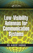
2.3.3 Dipole E-Plane Radiation Pattern

The dipole E-plane radiation pattern is given in Equation 2.14 and presented in Figure 2.2.

$\left|E_{\theta }\right|={\eta }_0\frac{l\beta I_0\left|\sin \theta \right|}{4\pi r}$ (2.14)

At a given point P(r, θ, φ) the dipole E-plane radiation pattern is given in Equation 2.15.

$\begin{array}{l}\left|E_{\theta }\right|={\eta }_0\frac{l\beta I_0\left|\sin \theta \right|}{4\pi r}=A\left|\sin \theta \right|\\ \begin{array}{cc}\text{Choose}& A=1\end{array}\\ \left|E_{\theta }\right|=\left|\sin \theta \right|\end{array}$ (2.15)

The dipole E-plane radiation pattern in spherical coordinate system is shown in Figure 2.3.

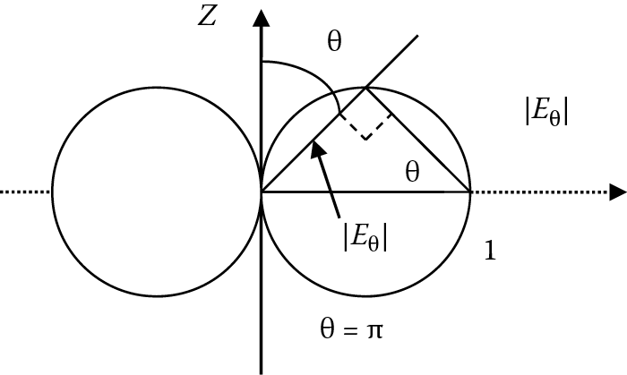
2.3.4 Dipole H-Plane Radiation Pattern

For θ = π/2 the dipole H-plane radiation pattern is given in Equation 2.10 and presented in Figure 2.4.

$\left|E_{\theta }\right|={\eta }_0\frac{l\beta I_0}{4\pi r}$ (2.16)

At a given point P(r, θ, φ) the dipole H-plane radiation pattern is given in Equation 2.17.

$\begin{array}{l}\left|E_{\theta }\right|={\eta }_0\frac{l\beta I_0\left|\sin \theta \right|}{4\pi r}=A\\ \begin{array}{cc}\text{Choose}& A=1\end{array}\\ \left|E_{\theta }\right|=1\end{array}$ (2.17)

The dipole H-plane radiation pattern in the x–y plane is a circle with r = 1.

The radiation pattern of a vertical dipole is omnidirectional. It radiates equal power in all azimuthal directions perpendicular to the axis of the antenna. The dipole H-plane radiation pattern in spherical coordinate system is shown in Figure 2.4.

2.3.5 Antenna Radiation Pattern

A typical antenna radiation pattern is shown in Figure 2.5. The antenna main beam is measured between the points that the maximum relative field intensity E decays to 0.707E. Half of the radiated power is concentrated in the antenna main beam. The antenna main beam is called the 3 dB beam width. Radiation to an undesired direction is concentrated in the antenna side lobes.

For a dipole the power intensity varies as (sin2 θ). At θ = 45° and θ = 135° the radiated power equals half the power radiated toward θ = 90°. The dipole beam width is

θ = (135 – 45) = 90°.

2.3.6 Dipole Directivity

Directivity is defined as the ratio between the amounts of energy propagating in a certain direction compared to the average energy radiated to all directions over a sphere as written in Equations 2.18 and 2.19.

$D=\frac{P\left(\theta ,\varphi \right)\text{maximal}}{P\left(\theta ,\varphi \right)\text{average}}=4\pi \frac{P\left(\theta ,\varphi \right)\text{maximal}}{P_{\text{rad}}}$ (2.18)

$P\left(\theta ,\varphi \right)\text{average}=\frac{1}{4\pi }{\displaystyle \iint P\left(\theta ,\varphi \right)\text{sin}\theta d\theta d\varphi =\frac{P_{\text{rad}}}{4\pi }}$ (2.19)

The radiated power from a dipole is calculated by computing the Poynting vector P as given in Equation 2.20.

$\begin{array}{l}P=0.5(E\times H*)=\frac{15\pi I_0^2{l}^2{\sin }^2\theta }{r^2{\lambda }^2}\\ W_T={\displaystyle \underset{s}{\int }P\cdot ds=\frac{15\pi I_0^2{l}^2}{{\lambda }^2}{\displaystyle \underset{0}{\overset{\pi }{\int }}{\sin }^3\theta d\theta {\displaystyle \underset{0}{\overset{2\pi }{\int }}d\varphi }}}=\frac{40{\pi }^2{I}_0^2{l}^2}{{\lambda }^2}\end{array}$ (2.20)

The overall radiated energy is WT. WT is computed by integration of the power flow over an imaginary sphere surrounding the dipole. The power flow of an isotropic radiator is equal to WT divided by the surrounding area of the sphere, 4πr2, as given in Equation 2.21. The dipole directivity at θ = 90° is 1.5 or 1.76 dB as shown in Equation 2.22.

$\begin{array}{l}{\displaystyle \underset{s}{\oint }ds=r^2{\displaystyle \underset{0}{\overset{\pi }{\int }}\sin \theta d\theta {\displaystyle \underset{0}{\overset{2\pi }{\int }}d\varphi }}}=4\pi r^2\\ P_{\text{iso}}=\frac{W_T}{4\pi r^2}=\frac{10\pi I_0^2{l}^2}{r^2{\lambda }^2}\\ D=\frac{P}{P_{\text{iso}}}=1.5{\sin }^2\theta \end{array}$ (2.21)

GdB = 10 log10 G = 10 log10 1.5 = 1.76 dB (2.22)

For small antennas or for antennas without losses, D = G, losses are negligible. For a given θ and φ for small antennas the approximate directivity is given by Equation 2.23.

$\begin{array}{l}D=\frac{41,253}{{\theta }_{3\text{dB}}{\phi }_{3\text{dB}}}\\ G=\xi D\xi =\text{Efficiency}\end{array}$ (2.23)

Antenna losses degrade the antenna efficiency. Antenna losses consist of conductor loss, dielectric loss, radiation loss, and mismatch losses. For resonant small antennas ξ = 1. For reflector and horn antennas the efficiency varies between ξ = 0.5 and ξ = 0.7.

2.3.7 Antenna Impedance

Antenna impedance determines the efficiency of transmitting and receiving energy in antennas. The dipole impedance is given in Equation 2.24.

$\begin{array}{l}{R}_{\text{rad}}=\frac{2W_T}{I_0^2}\\ \text{For}\text{a}\text{dipole}\\ R_{\text{rad}}=\frac{80{\pi }^2{l}^2}{{\lambda }^2}\end{array}$ (2.24)

2.3.8 Impedance of a Folded Dipole

A folded dipole is a half-wave dipole with an additional wire connecting its two ends. If the additional wire has the same diameter and cross section as the dipole, two nearly identical radiating currents are generated. The resulting far-field emission pattern is nearly identical to the one for the single-wire dipole described previously, but at resonance its feed point impedance Rrad−f is four times the radiation resistance of a dipole. This is because for a fixed amount of power, the total radiating current I0 is equal to twice the current in each wire and thus equal to twice the current at the feed point. Equating the average radiated power to the average power delivered at the feed point, we obtain that Rrad−f = 4 Rrad = 300 Ω. The folded dipole has a wider bandwidth than a single dipole.

2.4 Basic Aperture Antennas

Reflector and horn antennas are defined as aperture antennas. The longest dimension of an aperture antenna is greater than several wavelengths.

2.4.1 The Parabolic Reflector Antenna

The parabolic reflector antenna [3] consists of a radiating feed that is used to illuminate a reflector that is curved in the form of an accurate parabolic with diameter D as presented in Figure 2.6. This shape enables evert beam to be obtained. To provide the optimum illumination of the reflecting surface, the level of the parabola illumination should be greater by 10 dB in the center than that at the parabola edges. The parabolic reflector antenna gain may be calculated by using Equation 2.25. α is the parabolic reflector antenna efficiency.

Parabolic reflector antenna gain:

$G\cong 10{\text{log}}_{10}\left(\alpha \frac{{(\pi D)}^2}{{\lambda }^2}\right)$ (2.25)

Reflector geometry is presented in Figure 2.7.

The following relations given in Equations 2.26 to 2.29 can be derived from the reflector geometry.

PQ = rʹ cos θʹ (2.26)

2f = r′(1 + cos θ′) (2.27)

$2f=r^{\prime }+r^{\prime }\text{cos}{\theta }^{\prime }=\sqrt{{(x^{\prime })}^2+{(y^{\prime })}^2+{(z^{\prime })}^2}+z^{\prime }$ (2.28)

The relation between the reflector diameter D and θ is given in Equations 2.29 to 2.31.

${\theta }_0={\text{tan}}^{-1}\frac{\frac{D}{2}}{z_0}$ (2.29)

$z_0=f-\frac{{\left(\frac{D}{2}\right)}^2}{4f}$ (2.30)

${\theta }_0={\text{tan}}^{-1}\left|\frac{\frac{D}{2}}{z_0}\right|={\text{tan}}^{-1}\left|\frac{\frac{D}{2}}{f-\frac{{\left(\frac{D}{2}\right)}^2}{4f}}\right|={\text{tan}}^{-1}\left|\frac{\frac{f}{2D}}{{\left(\frac{f}{D}\right)}^2-\frac{1}{16}}\right|$ (2.31)

$f=\frac{D}{4}\text{cot}\left(\frac{{\theta }_0}{2}\right)$ (2.32)

2.4.2 Reflector Directivity

Reflector directivity is a function of the reflector geometry and feed radiation characteristics as given in Equations 2.33 and 2.34.

$D_0=\frac{4\pi U_{\text{max}}}{P_{\text{rad}}}=\frac{16{\pi }^2}{{\lambda }^2}{f}^2{\left|\underset{0}{\overset{{\theta }_0}{{\displaystyle \int }}}\sqrt{G_F({\theta }^{\prime })}tan\left(\frac{{\theta }^{\prime }}{2}\right)d{\theta }^{\prime }\right|}^2$ (2.33)

$D_0=\frac{{(\pi D)}^2}{{\lambda }^2}\left[{\text{cot}}^2\left(\frac{{\theta }_0}{2}\right){\left|{\displaystyle \underset{0}{\overset{{\theta }_0}{\int }}\sqrt{G_F({\theta }^{\prime })}\text{tan}\left(\frac{{\theta }^{\prime }}{2}\right)d{\theta }^{\prime }}\right|}^2\right]$ (2.34)

The reflector aperture efficiency is given in Equation 2.35. The feed radiation pattern may be presented as in Equation 2.36.

${ϵ}_{\text{ap}}=\left[{\text{cot}}^2\left(\frac{{\theta }_0}{2}\right){\left|{\displaystyle \underset{0}{\overset{{\theta }_0}{\int }}\sqrt{G_F({\theta }^{\prime })}\text{tan}\left(\frac{{\theta }^{\prime }}{2}\right)d{\theta }^{\prime }}\right|}^2\right]$ (2.35)

$\begin{array}{l}{G}_F({\theta }^{\prime })=G_0^n{\text{cos}}^n({\theta }^{\prime })\text{for}0\le {\theta }^{\prime }\le \frac{\pi }{2}\\ G_F({\theta }^{\prime })=0\text{for}\frac{\pi }{2}<{\theta }^{\prime }\le \pi \\ {\displaystyle \underset{0}{\overset{\pi \text{/}2}{\int }}{G}_0^n{\text{cos}}^n({\theta }^{\prime })\text{sin}({\theta }^{\prime })d{\theta }^{\prime }=2}\end{array}$ (2.36)

where

$G_0^n=2(n+1)$

Uniform illumination of the reflector aperture may be achieved if GF(θ′) is given by Equation 2.37.

$\begin{array}{l}{G}_F({\theta }^{\prime })={\text{sec}}^4\left(\frac{{\theta }^{\prime }}{2}\right)\text{for}0\le {\theta }^{\prime }\le \frac{\pi }{2}\\ G_F({\theta }^{\prime })=0\text{for}\frac{\pi }{2}<{\theta }^{\prime }\le \pi \end{array}$ (2.37)

The reflector aperture efficiency is computed by multiplying all the antenna efficiencies due to spillover, blockage, taper, phase error, cross polarization losses, and random error over the reflector surface.

${ϵ}_{\text{ap}}={ϵ}_{\text{s}}{ϵ}_{\text{t}}{ϵ}_{\text{b}}{ϵ}_{\text{x}}{ϵ}_{\text{p}}{ϵ}_{\text{r}}$

where

${ϵ}_{\text{s}}$ = spillover efficiency, written in Equation 2.38

${ϵ}_{\text{t}}$ = taper efficiency, written in Equation 2.39

${ϵ}_{\text{b}}$ = blockage efficiency

${ϵ}_{\text{p}}$ = phase efficiency

${ϵ}_{\text{x}}$ = cross polarization efficiency

${ϵ}_{\text{r}}$ = random error over the reflector surface efficiency

${ϵ}_{\text{s}}=\frac{{\displaystyle {\int }_0^{{\theta }_0}{G}_F({\theta }^{\prime })\text{sin}{\theta }^{\prime }d{\theta }^{\prime }}}{{\displaystyle {\int }_{\pi }^{{\theta }_0}{G}_F({\theta }^{\prime })\text{sin}{\theta }^{\prime }d{\theta }^{\prime }}}$ (2.38)

${ϵ}_{\text{t}}=2{\text{cot}}^2\left(\frac{{\theta }_0}{2}\right)\frac{{\left|{\displaystyle {\int }_0^{{\theta }_0}\sqrt{G_F({\theta }^{\prime })}\text{tan}\left(\frac{{\theta }^{\prime }}{2}\right)d{\theta }^{\prime }}\right|}^2}{{\displaystyle {\int }_0^{{\theta }_0}{G}_F({\theta }^{\prime })\text{sin}{\theta }^{\prime }d{\theta }^{\prime }}}$ (2.39)

In the literature [1] we can find graphs that present the reflector antenna efficiencies as a function of the reflector antenna geometry and feed radiation pattern. However, Equations 2.34 to 2.40 give us a good approximation of the reflector directivity.

$D_0=\frac{{(\pi D)}^2{ϵ}_{\text{ap}}}{{\lambda }^2}$ (2.40)

2.4.3 Cassegrain Reflector

The parabolic reflector or dish antenna consists of a radiating element that may be a simple dipole or a waveguide horn antenna. This is placed at the center of the metallic parabolic reflecting surface as shown in Figure 2.8. The energy from the radiating element is arranged so that it illuminates the subreflecting surface. The energy from the subreflector is arranged so that it illuminates the main reflecting surface. Once the energy is reflected it leaves the antenna system in a narrow beam.

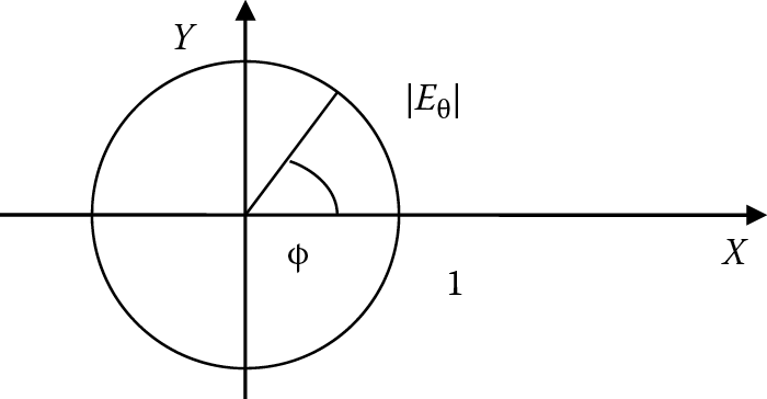
2.5 Horn Antennas

Horn antennas are used as a feed element for radio astronomy, satellite tracking and communication reflector antennas, and phased arrays radiating elements, used in antenna calibration and measurements. Figure 2.9 shows an E-plane sectoral horn. Figure 2.9 shows an H-plane sectoral horn. Figure 2.9 shows a pyramidal horn. Figure 2.9 shows a conical horn.

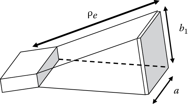
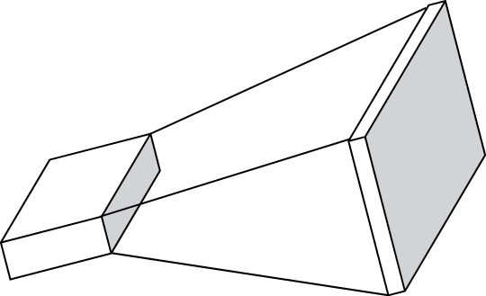
2.5.1 E-Plane Sectoral Horn

Figure 2.10 shows an E-plane sectoral horn. Horn antennas are fed by a waveguide. The excited mode is TE10. Fields expressions over the horn aperture are similar to the fields of a TE10 mode in a rectangular waveguide with the aperture dimensions of a, b1. The fields in the antenna aperture are given in Equations 2.41 to 2.43.

${E^{\prime }}_y(x^{\prime },y^{\prime })\approx E_1\cos \left(\frac{\pi }{a}{x}^{\prime }\right)e^{-j\left[k{y^{\prime }}^2/(2{\rho }_1)\right]}$ (2.41)

${H^{\prime }}_x(x^{\prime },y^{\prime })\approx \frac{E_1}{\eta }\cos \left(\frac{\pi }{a}{x}^{\prime }\right)e^{-j\left[k{y^{\prime }}^2/(2{\rho }_1)\right]}$ (2.42)

${H^{\prime }}_z(x^{\prime },y^{\prime })\approx j{E}_1\left(\frac{\pi }{ka\eta }\right)\sin \left(\frac{\pi }{a}{x}^{\prime }\right)e^{-j\left[k{y^{\prime }}^2/(2{\rho }_1)\right]}$ (2.43)

The horn length is ρ1, as shown in Figure 2.11. The extra distance along the aperture sides compared with the distance to the center is δ and is given by Equation 2.44.

$\delta ={\rho }_e-\sqrt{{\rho }_e-{\left(\frac{b_1}{2}\right)}^2}={\rho }_e(1-\sqrt{1-{\left(\frac{b_1}{2{\rho }_e}\right)}^2}=\frac{b_1^2}{8{\rho }_e}$ (2.44)

$\frac{\delta }{\lambda }=S=\frac{b_1^2}{8\lambda {\rho }_e}$ (2.45)

S represents the quadratic phase distribution as given in Equation 2.45.

${(\delta (y^{\prime })+{\rho }_1)}^2={\rho }_1^2+{(y^{\prime })}^2$ (2.46)

$\delta (y^{\prime })=-{\rho }_1+\sqrt{{\rho }_1^2+{(y^{\prime })}^2}=-{\rho }_1+{\rho }_1\sqrt{1+{\left(\frac{y^{\prime }}{{\rho }_1}\right)}^2}$ (2.47)

The maximum phase deviation at the aperture ∅max is given by Equation 2.48.

${\varnothing }_{\text{max}}=k\delta (y^{\prime })⋮\left(y^{\prime }=\frac{b_1}{2}\right)=\frac{k{b}_1^2}{8{\rho }_1}$ (2.48)

The total flare angle of the horn, 2ψe, is given in Equation 2.49.

$2{\psi }_e=2{\text{tan}}^{-1}\left(\frac{b_1}{2{\rho }_1}\right)$ (2.49)

Directivity of the E-Plane Horn

The maximum radiation is given by Equation 2.50.

$U_{\text{max}}=\frac{r^2}{2\eta }{\left|E\right|}_{\text{max}}^2$ (2.50)

$U_{\text{max}}=\frac{2k{a}^2{\rho }_1}{{\pi }^3\eta }{\left|E\right|}^2{\left|F(t)\right|}^2$ (2.51)

${\left|F(t)\right|}^2=\left[C^2\left(\frac{b_1}{\sqrt{2\lambda {\rho }_1}}\right)+S^2\left(\frac{b_1}{\sqrt{2\lambda {\rho }_1}}\right)\right]$ (2.52)

C and S are Fresnel integers and are given in Table 2.2. The total radiated power by the horn is given in Equation 2.53.

$P_{\text{rad}}=\frac{a{b}_1}{4\eta }{\left|E\right|}^2$ (2.53)

The directivity of E-plane horn DE is given in Equation 2.54.

$D_E=\frac{4\pi U_{\text{max}}}{P_{\text{rad}}}=\frac{64a{\rho }_1}{\pi \lambda b_1}\left[C^2\left(\frac{b_1}{\sqrt{2\lambda {\rho }_1}}\right)+S^2\left(\frac{b_1}{\sqrt{2\lambda {\rho }_1}}\right)\right]$ (2.54)

Figure 2.12 presents the H-plane horn radiation pattern as function of S,

where $S=\frac{b_1^2}{8\lambda {\rho }_e}$ .

2.5.2 H-Plane Sectoral Horn

An H-plane sectoral horn is shown in Figure 2.13. H-plane sectoral horn geometry is shown in Figure 2.14. Fields expressions over the horn aperture are similar to the fields of a TE10 mode in rectangular waveguide with the aperture dimensions of a, b1. The fields in the antenna aperture are written in Equations 2.55 and 2.56.

${E^{\prime }}_y(x^{\prime },y^{\prime })\approx E_2\cos \left(\frac{\pi }{a}{x}^{\prime }\right)e^{-j\left[k{x^{\prime }}^2/(2{\rho }_2)\right]}$ (2.55)

${H^{\prime }}_x(x^{\prime },y^{\prime })\approx \frac{E_2}{\eta }\cos \left(\frac{\pi }{a}{x}^{\prime }\right)e^{-j\left[k{x^{\prime }}^2/(2{\rho }_2)\right]}$ (2.56)

The horn length is ρl. The extra distance along the aperture sides compared with the distance to the center is δ and is given by Equation 2.57.

$\delta ={\rho }_h-\sqrt{{\rho }_h-{\left(\frac{a_1}{2}\right)}^2}={\rho }_h(1-\sqrt{1-{\left(\frac{a_1}{2{\rho }_h}\right)}^2}=\frac{a_1^2}{8{\rho }_h}$ (2.57)

$\frac{\delta }{\lambda }=S=\frac{a_1^2}{8\lambda {\rho }_h}$ (2.58)

S represents the quadratic phase distribution as written in Equation 2.58.

${(\delta (x^{\prime })+{\rho }_2)}^2={\rho }_2^2+{(x^{\prime })}^2$ (2.59)

$\delta (x^{\prime })=-{\rho }_2+\sqrt{{\rho }_2^2+{(x^{\prime })}^2}=-{\rho }_2+{\rho }_1\sqrt{1+{\left(\frac{x^{\prime }}{{\rho }_2}\right)}^2}$ (2.60)

The maximum phase deviation at the aperture ∅max is given by Equation 2.61.

${\varnothing }_{\text{max}}=k\delta (x^{\prime })⋮\left(x^{\prime }=\frac{a_1}{2}\right)=\frac{k{a}_1^2}{8{\rho }_2}$ (2.61)

The total flare angle of the horn, 2ψe, is given in Equation 2.62.

$2{\psi }_h=2{\text{tan}}^{-1}\left(\frac{a_1}{2{\rho }_2}\right)$ (2.62)

Directivity of the E-Plane Horn

The maximum radiation is given by Equations 2.63 and 2.64.

$U_{\text{max}}=\frac{r^2}{2\eta }{\left|E\right|}_{\text{max}}^2$ (2.63)

$U_{\text{max}}=\frac{b^2{\rho }_2}{4\lambda \eta }{\left|E\right|}^2{\left|F(t)\right|}^2$ (2.64)

|F(t)|2 = [(C(u) − C(v))2 + (S(u) − S(v))2] (2.65)

where $u=\frac{1}{\sqrt{2}}\left(\frac{\sqrt{{\rho }_2\lambda }}{a_1}-\frac{a_1}{\sqrt{{\rho }_2\lambda }}\right)$ and $v=\frac{1}{\sqrt{2}}\left(\frac{\sqrt{{\rho }_2\lambda }}{a_1}+\frac{a_1}{\sqrt{{\rho }_2\lambda }}\right)$

C and S are Fresnel integers. The total radiated power by the horn is given in Equation 2.66.

$P_{\text{rad}}=\frac{a{b}_1}{4\eta }{\left|E\right|}^2$ (2.66)

The directivity of H-plane horn DH is given in Equation 2.67.

$D_H=\frac{4\pi U_{\text{max}}}{P_{\text{rad}}}=\frac{4b\pi {\rho }_2}{\lambda a_1}{[{(C(u)-C(v))}^2+(S(u)-S(v))]}^2$ (2.67)

An H-plane horn radiation pattern as a function of S, $S=\frac{a_1^2}{8\lambda {\rho }_h}$ , is shown in Figure 2.15.

2.5.3 Pyramidal Horn Antenna

The pyramidal horn antenna is a combination of the E and H horns as shown in Figure 2.16. The pyramidal horn antenna is realizable only if ρh = ρe.

The directivity of pyramidal horn antenna DP is given in Equation 2.68.

$D_P=\frac{4\pi U_{max}}{P_{rad}}=\frac{\pi {\lambda }^2}{32ab}{D}_E{D}_H$ (2.68)

Kraus [3] gives the following approximation for pyramidal horn beam width.

${\theta }_{3\text{dB}}^e=\frac{56}{A_{e\lambda }}$ (2.69)

${\theta }_{3\text{dB}}^h=\frac{67}{A_{h\lambda }}$ (2.70)

${\theta }_{10\text{dB}}^e=\frac{100.8}{A_{e\lambda }}$ (2.71)

${\theta }_{10\text{dB}}^h=\frac{120.6}{A_{h\lambda }}$ (2.72)

Aeλ is the aperture dimensions in wavelength in the the E plane. Ahλ is the aperture dimensions in wavelength in the H plane. The pyramidal horn gain is given by Equation 2.73.

G = 10log10 4.5AhλAeλ dBi (2.73)

The relative power at any angle, $P_{\text{dB}}^h(\theta )$ , is given approximately by Equation 2.74.

$P_{\text{dB}}^h(\theta )=10{\left(\frac{\theta }{{\theta }_{10\text{dB}}^h}\right)}^2$ (2.74)

References

1. Balanis, C. A. Antenna Theory: Analysis and Design, 2nd ed. New York: John Wiley & Sons, 1996

2. Godara, L. C. (Ed.). Handbook of Antennas in Wireless Communications. Boca Raton, FL: CRC Press, 2002.

3. Kraus, J. D., and Marhefka, R. J. Antennas for All Applications, 3rd ed. New York: McGraw-Hill, 2002.

4. James, J. R., Hall, P. S., and Wood, C. Microstrip Antenna Theory and Design. London: The Institution of Engineering and Technology, 1981.

5. Sabban, A., and Gupta, K. C. Characterization of Radiation Loss from Microstrip Discontinuities Using a Multiport Network Modeling Approach. IEEE Transactions on Microwave Theory and Techniques, 39(4): 705–712, 1991.

6. Sabban, A. Multiport Network Model for Evaluating Radiation Loss and Coupling Among Discontinuities in Microstrip Circuits. PhD thesis, University of Colorado at Boulder, January 1991.

7. Kathei, P. B., and Alexopoulos, N. G. Frequency-Dependent Characteristic of Microstrip, Discontinuities in Millimeter-Wave Integrated Circuits. IEEE Transactions on Microwave Theory and Techniques, 33: 1029–1035, 1985.

8. Sabban, A. A New Wideband Stacked Microstrip Antenna. In IEEE Antenna and Propagation Symposium, Houston, TX, June 1983.

9. Sabban, A., and Navon, E. A MM-Waves Microstrip Antenna Array. In IEEE Symposium, Tel Aviv, Israel, March 1983.

10. Sabban, A. Wideband Microstrip Antenna Arrays. In IEEE Antenna and Propagation Symposium MELCOM, Tel Aviv, Israel, June 1981.

11. Sabban, A. RF Engineering, Microwave and Antennas. Tel Aviv, Israel: Saar Publication, 2014.