
Routine breast cancer screening allows the disease to be diagnosed and treated prior to it causing noticeable symptoms. The process of early detection involves examining the breast tissue for abnormal lumps or masses. If a lump is found, a fine-needle aspiration biopsy is performed, which uses a hollow needle to extract a small sample of cells from the mass. A clinician then examines the cells under a microscope to determine whether the mass is likely to be malignant or benign.
If machine learning could automate the identification of cancerous cells, it would provide considerable benefit to the health system. Automated processes are likely to improve the efficiency of the detection process, allowing physicians to spend less time diagnosing and more time treating the disease. An automated screening system might also provide greater detection accuracy by removing the inherently subjective human component from the process.
We will investigate the utility of machine learning for detecting cancer by applying the k-NN algorithm to measurements of biopsied cells from women with abnormal breast masses.
We will utilize the Breast Cancer Wisconsin (Diagnostic) dataset from the UCI Machine Learning Repository at http://archive.ics.uci.edu/ml. This data was donated by researchers of the University of Wisconsin and includes measurements from digitized images of fine-needle aspirate of a breast mass. The values represent characteristics of the cell nuclei present in the digital image.
The breast cancer data includes 569 examples of cancer biopsies, each with 32 features. One feature is an identification number, another is the cancer diagnosis, and 30 are numeric-valued laboratory measurements. The diagnosis is coded as "M" to indicate malignant or "B" to indicate benign.
The 30 numeric measurements comprise the mean, standard error, and worst (that is, largest) value for 10 different characteristics of the digitized cell nuclei. These include:
- Radius
- Texture
- Perimeter
- Area
- Smoothness
- Compactness
- Concavity
- Concave points
- Symmetry
- Fractal dimension
Based on these names, all features seem to relate to the shape and size of the cell nuclei. Unless you are an oncologist, you are unlikely to know how each relates to benign or malignant masses. These patterns will be revealed as we continue in the machine learning process.
Let's explore the data and see if we can shine some light on the relationships. In doing so, we will prepare the data for use with the k-NN learning method.
We'll begin by importing the CSV data file as we have done in previous chapters, saving the Wisconsin breast cancer data to the wbcd data frame:
> wbcd <- read.csv("wisc_bc_data.csv", stringsAsFactors = FALSE)
Using the command str(wbcd), we can confirm that the data is structured with 569 examples and 32 features, as we expected. The first several lines of output are as follows:
'data.frame':  569 obs. of  32 variables:
 $ id               : int  87139402 8910251 905520 ...
 $ diagnosis        : chr  "B" "B" "B" "B" ...
 $ radius_mean      : num  12.3 10.6 11 11.3 15.2 ...
 $ texture_mean     : num  12.4 18.9 16.8 13.4 13.2 ...
 $ perimeter_mean   : num  78.8 69.3 70.9 73 97.7 ...
 $ area_mean        : num  464 346 373 385 712 ...
The first variable is an integer variable named id. As this is simply a unique identifier (ID) for each patient in the data, it does not provide useful information and we will need to exclude it from the model.
Tip
Regardless of the machine learning method, ID variables should always be excluded. Neglecting to do so can lead to erroneous findings because the ID can be used to correctly predict each example. Therefore, a model that includes an ID column will almost definitely suffer from overfitting and generalize poorly to future data.
Let's drop the id feature altogether. As it is located in the first column, we can exclude it by making a copy of the wbcd data frame without column 1:
> wbcd <- wbcd[-1]
The next variable, diagnosis, is of particular interest as it is the outcome we hope to predict. This feature indicates whether the example is from a benign or malignant mass. The table() output indicates that 357 masses are benign, while 212 are malignant:
> table(wbcd$diagnosis)
    B   M
357 212
Many R machine learning classifiers require the target feature to be coded as a factor, so we will need to recode the diagnosis variable. We will also take this opportunity to give the "B" and "M" values more informative labels using the labels parameter:
> wbcd$diagnosis <- factor(wbcd$diagnosis, levels = c("B", "M"),labels = c("Benign", "Malignant"))
When we look at the prop.table() output, we now find that the values have been labeled Benign and Malignant, with 62.7 percent and 37.3 percent of the masses, respectively:
> round(prop.table(table(wbcd$diagnosis)) * 100, digits = 1)
   Benign Malignant
     62.7      37.3
The remaining 30 features are all numeric and, as expected, consist of three different measurements of 10 characteristics. For illustrative purposes, we will only take a closer look at three of these features:
> summary(wbcd[c("radius_mean", "area_mean", "smoothness_mean")])
  radius_mean       area_mean      smoothness_mean
 Min.   : 6.981   Min.   : 143.5   Min.   :0.05263
 1st Qu.:11.700   1st Qu.: 420.3   1st Qu.:0.08637
 Median :13.370   Median : 551.1   Median :0.09587
 Mean   :14.127   Mean   : 654.9   Mean   :0.09636
 3rd Qu.:15.780   3rd Qu.: 782.7   3rd Qu.:0.10530
 Max.   :28.110   Max.   :2501.0   Max.   :0.16340
Looking at the three side-by-side, do you notice anything problematic about the values? Recall that the distance calculation for k-NN is heavily dependent upon the measurement scale of the input features. Since smoothness ranges from 0.05 to 0.16, while area ranges from 143.5 to 2501.0, the impact of area is going to be much greater than smoothness in the distance calculation. This could potentially cause problems for our classifier, so let's apply normalization to rescale the features to a standard range of values.
To normalize these features, we need to create a normalize() function in R. This function takes a vector x of numeric values, and for each value in x, subtracts the minimum x value and divides by the range of x values. Lastly, the resulting vector is returned. The code for the function is as follows:
> normalize <- function(x) {
      return ((x - min(x)) / (max(x) - min(x)))
    }
After executing the previous code, the normalize() function is available for use in R. Let's test the function on a couple of vectors:
> normalize(c(1, 2, 3, 4, 5))
[1] 0.00 0.25 0.50 0.75 1.00
> normalize(c(10, 20, 30, 40, 50))
[1] 0.00 0.25 0.50 0.75 1.00
The function appears to be working correctly. Despite the fact that the values in the second vector are 10 times larger than the first vector, after normalization, they both appear exactly the same.
We can now apply the normalize() function to the numeric features in our data frame. Rather than normalizing each of the 30 numeric variables individually, we will use one of R's functions to automate the process.
The lapply() function takes a list and applies a specified function to each list element. As a data frame is a list of equal-length vectors, we can use lapply() to apply normalize() to each feature in the data frame. The final step is to convert the list returned by lapply() to a data frame using the as.data.frame() function. The full process looks like this:
> wbcd_n <- as.data.frame(lapply(wbcd[2:31], normalize))
In plain English, this command applies the normalize() function to columns 2 to 31 in the wbcd data frame, converts the resulting list to a data frame, and assigns it the name wbcd_n. The _n suffix is used here as a reminder that the values in wbcd have been normalized.
To confirm that the transformation was applied correctly, let's look at one variable's summary statistics:
> summary(wbcd_n$area_mean)
Min.    1st Qu. Median  Mean    3rd Qu. Max.
0.0000  0.1174  0.1729  0.2169  0.2711  1.0000
As expected, the area_mean variable, which originally ranged from 143.5 to 2501.0, now ranges from 0 to 1.
Although all 569 biopsies are labeled with a benign or malignant status, it is not very interesting to predict what we already know. Additionally, any performance measures we obtain during training may be misleading, as we do not know the extent to which the data has been overfitted or how well the learner will generalize to new cases. For these reasons, a more interesting question is how well our learner performs on a dataset of unseen data. If we had access to a laboratory, we could apply our learner to measurements taken from the next 100 masses of unknown cancer status and see how well the machine learner's predictions compare to diagnoses obtained using conventional methods.
In the absence of such data, we can simulate this scenario by dividing our data into two portions: a training dataset that will be used to build the k-NN model and a test dataset that will be used to estimate the predictive accuracy of the model. We will use the first 469 records for the training dataset and the remaining 100 to simulate new patients.
Using the data extraction methods presented in Chapter 2, Managing and Understanding Data, we will split the wbcd_n data frame into wbcd_train and wbcd_test:
> wbcd_train <- wbcd_n[1:469, ]
> wbcd_test <- wbcd_n[470:569, ]
If the previous commands are confusing, remember that data is extracted from data frames using the [row, column] syntax. A blank value for the row or column value indicates that all rows or columns should be included. Hence, the first line of code requests rows 1 to 469 and all columns, and the second line requests 100 rows from 470 to 569 and all columns.
Tip
When constructing training and test datasets, it is important that each dataset is a representative subset of the full set of data. The wbcd records were already randomly ordered, so we could simply extract 100 consecutive records to create a test dataset. This would not be appropriate if the data was ordered chronologically or in groups of similar values. In these cases, random sampling methods would be needed. Random sampling will be discussed in Chapter 5, Divide and Conquer – Classification Using Decision Trees and Rules.
When we constructed our normalized training and test datasets, we excluded the target variable, diagnosis. For training the k-NN model, we will need to store these class labels in factor vectors, split between the training and test datasets:
> wbcd_train_labels <- wbcd[1:469, 1]
> wbcd_test_labels <- wbcd[470:569, 1]
This code takes the diagnosis factor in the first column of the wbcd data frame and creates the vectors wbcd_train_labels and wbcd_test_labels. We will use these in the next steps of training and evaluating our classifier.
Equipped with our training data and vector of labels, we are now ready to classify our test records. For the k-NN algorithm, the training phase actually involves no model building; the process of training a lazy learner like k-NN simply involves storing the input data in a structured format.
To classify our test instances, we will use a k-NN implementation from the class package, which provides a set of basic R functions for classification. If this package is not already installed on your system, you can install it by typing:
> install.packages("class")
To load the package during any session in which you wish to use the functions, simply enter the library(class) command.
The knn() function in the class package provides a standard, classic implementation of the k-NN algorithm. For each instance in the test data, the function will identify the k nearest neighbors, using Euclidean distance, where k is a user-specified number. The test instance is classified by taking a "vote" among the k nearest neighbors—specifically, this involves assigning the class of the majority of the neighbors. A tie vote is broken at random.
Training and classification using the knn() function is performed in a single command with four parameters, as shown in the following table:

We now have nearly everything we need to apply the k-NN algorithm to this data. We've split our data into training and test datasets, each with exactly the same numeric features. The labels for the training data are stored in a separate factor vector. The only remaining parameter is k, which specifies the number of neighbors to include in the vote.
As our training data includes 469 instances, we might try k = 21, an odd number roughly equal to the square root of 469. With a two-category outcome, using an odd number eliminates the chance of ending with a tie vote.
Now we can use the knn() function to classify the test data:
> wbcd_test_pred <- knn(train = wbcd_train, test = wbcd_test,
                        cl = wbcd_train_labels, k = 21)
The knn() function returns a factor vector of predicted labels for each of the examples in the wbcd_test dataset. We have assigned these predictions to wbcd_test_pred.
The next step of the process is to evaluate how well the predicted classes in the wbcd_test_pred vector match the actual values in the wbcd_test_labels vector. To do this, we can use the CrossTable() function in the gmodels package, which was introduced in Chapter 2, Managing and Understanding Data. If you haven't done so already, please install this package using the install.packages("gmodels") command.
After loading the package with the library(gmodels) command, we can create a cross tabulation indicating the agreement between the predicted and actual label vectors. Specifying prop.chisq = FALSE will remove the unnecessary chi-square values from the output:
> CrossTable(x = wbcd_test_labels, y = wbcd_test_pred,
             prop.chisq = FALSE)
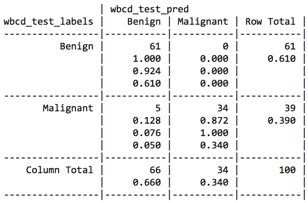
The resulting table looks like this:

The cell percentages in the table indicate the proportion of values that fall into four categories. The top-left cell indicates the true negative results. These 61 of 100 values are cases where the mass was benign and the k-NN algorithm correctly identified it as such. The bottom-right cell indicates the true positive results, where the classifier and the clinically determined label agree that the mass is malignant. A total of 37 of 100 predictions were true positives.
The cells falling on the other diagonal contain counts of examples where the k-NN prediction disagreed with the true label. The two examples in the lower-left cell are false negative results; in this case, the predicted value was benign, but the tumor was actually malignant. Errors in this direction could be extremely costly, as they might lead a patient to believe that she is cancer-free, but in reality, the disease may continue to spread.
The top-right cell would contain the false positive results, if there were any. These values occur when the model has classified a mass as malignant when in reality it was benign. Although such errors are less dangerous than a false negative result, they should also be avoided, as they could lead to additional financial burden on the health care system or stress for the patient, as unnecessary tests or treatment may be provided.
Tip
If we desired, we could totally eliminate false negatives by classifying every mass as malignant. Obviously, this is not a realistic strategy. Still, it illustrates the fact that prediction involves striking a balance between the false positive rate and the false negative rate. In Chapter 10, Evaluating Model Performance, you will learn methods for evaluating predictive accuracy that can be used to optimize performance to the costs of each type of error.
A total of 2 out of 100, or 2 percent of masses were incorrectly classified by the k-NN approach. While 98 percent accuracy seems impressive for a few lines of R code, we might try another iteration of the model to see if we can improve the performance and reduce the number of values that have been incorrectly classified, especially because the errors were dangerous false negatives.
We will attempt two simple variations on our previous classifier. First, we will employ an alternative method for rescaling our numeric features. Second, we will try several different k values.
Although normalization is commonly used for k-NN classification, z-score standardization may be a more appropriate way to rescale the features in a cancer dataset. Since z-score standardized values have no predefined minimum and maximum, extreme values are not compressed towards the center. Even in the absence of formal medical-domain training, one might suspect that a malignant tumor might lead to extreme outliers as tumors grow uncontrollably. With this in mind, it might be reasonable to allow the outliers to be weighted more heavily in the distance calculation. Let's see whether z-score standardization improves our predictive accuracy.
To standardize a vector, we can use R's built-in scale() function, which by default rescales values using the z-score standardization. The scale() function can be applied directly to a data frame, so there is no need to use the lapply() function. To create a z-score standardized version of the wbcd data, we can use the following command:
> wbcd_z <- as.data.frame(scale(wbcd[-1]))
This rescales all features with the exception of diagnosis in the first column and stores the result as the wbcd_z data frame. The _z suffix is a reminder that the values were z-score transformed.
To confirm that the transformation was applied correctly, we can look at the summary statistics:
> summary(wbcd_z$area_mean)
Min.     1st Qu.  Median   Mean    3rd Qu. Max.
-1.4530  -0.6666  -0.2949  0.0000  0.3632  5.2460
The mean of a z-score standardized variable should always be zero, and the range should be fairly compact. A z-score greater than 3 or less than -3 indicates an extremely rare value. Examining the summary statistics with these criteria in mind, the transformation seems to have worked.
As we have done before, we need to divide the z-score-transformed data into training and test sets, and classify the test instances using the knn() function. We'll then compare the predicted labels to the actual labels using CrossTable():
> wbcd_train <- wbcd_z[1:469, ]
> wbcd_test <- wbcd_z[470:569, ]
> wbcd_train_labels <- wbcd[1:469, 1]
> wbcd_test_labels <- wbcd[470:569, 1]
> wbcd_test_pred <- knn(train = wbcd_train, test = wbcd_test,
                        cl = wbcd_train_labels, k = 21)
> CrossTable(x = wbcd_test_labels, y = wbcd_test_pred,
             prop.chisq = FALSE)
Unfortunately, in the following table, the results of our new transformation show a slight decline in accuracy. Using the same instances in which we had previously classified 98 percent of examples correctly, we now classified only 95 percent correctly. Making matters worse, we did no better at classifying the dangerous false negatives.
We may be able to optimize the performance of the k-NN model by examining its performance across various k values. Using the normalized training and test datasets, the same 100 records were classified using several different choices of k. The number of false negatives and false positives are shown for each iteration:
|
k value |
False negatives |
False positives |
Percent classified incorrectly |
|---|---|---|---|
|
1 |
1 |
3 |
4 percent |
|
5 |
2 |
0 |
2 percent |
|
11 |
3 |
0 |
3 percent |
|
15 |
3 |
0 |
3 percent |
|
21 |
2 |
0 |
2 percent |
|
27 |
4 |
0 |
4 percent |
Although the classifier was never perfect, the 1-NN approach was able to avoid some of the false negatives at the expense of adding false positives. It is important to keep in mind, however, that it would be unwise to tailor our approach too closely to our test data; after all, a different set of 100 patient records is likely to be somewhat different from those used to measure our performance.
Tip
If you need to be certain that a learner will generalize to future data, you might create several sets of 100 patients at random and repeatedly retest the result. Such methods to carefully evaluate the performance of machine learning models will be discussed further in Chapter 10, Evaluating Model Performance.