Classification rule learning algorithms utilize a heuristic known as separate and conquer. The process involves identifying a rule that covers a subset of examples in the training data and then separating this partition from the remaining data. As rules are added, additional subsets of data are separated until the entire dataset has been covered and no more examples remain. Although separate and conquer is in many ways similar to the divide and conquer heuristic covered earlier, it differs in subtle ways that will become clear soon.

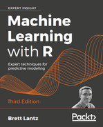
One way to imagine the rule learning process of separate and conquer is to imagine drilling down into the data by creating increasingly specific rules to identify class values. Suppose you were tasked with creating rules to identify whether or not an animal is a mammal. You could depict the set of all animals as a large space, as shown in the following diagram:

Figure 5.7: A rule learning algorithm may help divide animals into groups of mammals and non-mammals

A rule learner begins by using the available features to find homogeneous groups. For example, using a feature that indicates whether the species travels via land, sea, or air, the first rule might suggest that any land-based animals are mammals:

Figure 5.8: A potential rule considers animals that travel on land to be mammals

Do you notice any problems with this rule? If you're an animal lover, you might have realized that frogs are amphibians, not mammals. Therefore, our rule needs to be a bit more specific. Let's drill down further by suggesting that mammals must walk on land and have a tail:

Figure 5.9: A more specific rule suggests that animals that walk on land and have tails are mammals

As shown in the previous figure, the new rule results in a subset of animals that are entirely mammals. Thus, the subset of mammals can be separated from the other data and the frogs are returned to the pool of remaining animals—no pun intended!

An additional rule can be defined to separate out the bats, the only remaining mammal. A potential feature distinguishing bats from the remaining animals would be the presence of fur. Using a rule built around this feature, we have then correctly identified all the animals:

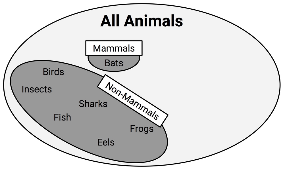
Figure 5.10: A rule stating that animals with fur are mammals perfectly classifies the remaining animals

At this point, since all of the training instances have been classified, the rule learning process would stop. We learned a total of three rules:

The previous example illustrates how rules gradually consume larger and larger segments of data to eventually classify all instances. As the rules seem to cover portions of the data, separate and conquer algorithms are also known as covering algorithms, and the resulting rules are called covering rules. In the next section, we will learn how covering rules are applied in practice by examining a simple rule learning algorithm. We will then examine a more complex rule learner and apply both algorithms to a real-world problem.

Suppose a television game show has an animal hidden behind a large curtain. You are asked to guess whether or not it is a mammal and if correct, you win a large cash prize. You are not given any clues about the animal's characteristics, but you know that a very small portion of the world's animals are mammals. Consequently, you guess "non-mammal." What do you think about your chances?

Choosing this, of course, maximizes your odds of winning the prize, as it is the most likely outcome under the assumption the animal was chosen at random. Clearly, this game show is a bit ridiculous, but it demonstrates the simplest classifier, ZeroR, which is a rule learner that considers no features and literally learns no rules (hence the name). For every unlabeled example, regardless of the values of its features, it predicts the most common class. This algorithm has very little real-world utility, except that it provides a simple baseline for comparison to other, more sophisticated, rule learners.

The 1R algorithm (One Rule or OneR), improves over ZeroR by selecting a single rule. Although this may seem overly simplistic, it tends to perform better than you might expect. As demonstrated in empirical studies, the accuracy of this algorithm can approach that of much more sophisticated algorithms for many real-world tasks.

The strengths and weaknesses of the 1R algorithm are shown in the following table:

The way this algorithm works is simple. For each feature, 1R divides the data into groups with similar values of the feature. Then, for each segment, the algorithm predicts the majority class. The error rate for the rule based on each feature is calculated and the rule with the fewest errors is chosen as the one rule.

The following tables show how this would work for the animal data we looked at earlier:

Figure 5.11: The 1R algorithm chooses the single rule with the lowest misclassification rate

For the Travels By feature, the dataset was divided into three groups: Air, Land, and Sea. Animals in the Air and Sea groups were predicted to be non-mammal, while animals in the Land group were predicted to be mammals. This resulted in two errors: bats and frogs.

The Has Fur feature divided animals into two groups. Those with fur were predicted to be mammals, while those without fur were not. Three errors were counted: pigs, elephants, and rhinos. As the Travels By feature resulted in fewer errors, the 1R algorithm would return the following:

The algorithm stops here, having found the single most important rule.

Obviously, this rule learning algorithm may be too basic for some tasks. Would you want a medical diagnosis system to consider only a single symptom, or an automated driving system to stop or accelerate your car based on only a single factor? For these types of tasks, a more sophisticated rule learner might be useful. We'll learn about one in the following section.

Early rule learning algorithms were plagued by a couple of problems. First, they were notorious for being slow, which made them ineffective for the increasing number of large datasets. Secondly, they were often prone to being inaccurate on noisy data.

A first step toward solving these problems was proposed in 1994 by Johannes Furnkranz and Gerhard Widmer. Their incremental reduced error pruning (IREP) algorithm uses a combination of pre-pruning and post-pruning methods that grow very complex rules and prune them before separating the instances from the full dataset. Although this strategy helped the performance of rule learners, decision trees often still performed better.

Rule learners took another step forward in 1995 when William W. Cohen introduced the repeated incremental pruning to produce error reduction (RIPPER) algorithm, which improved upon IREP to generate rules that match or exceed the performance of decision trees.

As outlined in the following table, the strengths and weaknesses of RIPPER are generally comparable to decision trees. The chief benefit is that they may result in a slightly more parsimonious model.

Having evolved from several iterations of rule learning algorithms, the RIPPER algorithm is a patchwork of efficient heuristics for rule learning. Due to its complexity, a discussion of the implementation details is beyond the scope of this book. However, it can be understood in general terms as a three-step process:

The growing phase uses the separate and conquer technique to greedily add conditions to a rule until it perfectly classifies a subset of data or runs out of attributes for splitting. Similar to decision trees, the information gain criterion is used to identify the next splitting attribute. When increasing a rule's specificity no longer reduces entropy, the rule is immediately pruned. Steps one and two are repeated until reaching a stopping criterion, at which point the entire set of rules is optimized using a variety of heuristics.

The RIPPER algorithm can create much more complex rules than the 1R algorithm can, as it can consider more than one feature. This means that it can create rules with multiple antecedents such as "if an animal flies and has fur, then it is a mammal." This improves the algorithm's ability to model complex data, but just like decision trees, it means that the rules can quickly become difficult to comprehend.

Classification rules can also be obtained directly from decision trees. Beginning at a leaf node and following the branches back to the root, you will have obtained a series of decisions. These can be combined into a single rule. The following figure shows how rules could be constructed from the decision tree for predicting movie success:

Figure 5.12: Rules can be generated from decision trees by following paths from the root node to each leaf node

Following the paths from the root node down to each leaf, the rules would be:

For reasons that will be made clear in the following section, the chief downside to using a decision tree to generate rules is that the resulting rules are often more complex than those learned by a rule learning algorithm. The divide and conquer strategy employed by decision trees biases the results differently to that of a rule learner. On the other hand, it is sometimes more computationally efficient to generate rules from trees.

Decision trees and rule learners are known as greedy learners because they use data on a first-come, first-served basis. Both the divide and conquer heuristic used by decision trees and the separate and conquer heuristic used by rule learners attempt to make partitions one at a time, finding the most homogeneous partition first, followed by the next best, and so on, until all examples have been classified.

The downside to the greedy approach is that greedy algorithms are not guaranteed to generate the optimal, most accurate, or smallest number of rules for a particular dataset. By taking the low-hanging fruit early, a greedy learner may quickly find a single rule that is accurate for one subset of data; however, in doing so, the learner may miss the opportunity to develop a more nuanced set of rules with better overall accuracy on the entire set of data. However, without using the greedy approach to rule learning, it is likely that for all but the smallest of datasets, rule learning would be computationally infeasible.

Figure 5.13: Both decision trees and classification rule learners are greedy algorithms

Though both trees and rules employ greedy learning heuristics, there are subtle differences in how they build rules. Perhaps the best way to distinguish them is to note that once divide and conquer splits on a feature, the partitions created by the split may not be re-conquered, only further subdivided. In this way, a tree is permanently limited by its history of past decisions. In contrast, once separate and conquer finds a rule, any examples not covered by all of the rule's conditions may be re-conquered.

To illustrate this contrast, consider the previous case in which we built a rule learner to determine whether an animal was a mammal. The rule learner identified three rules that perfectly classify the example animals:

In contrast, a decision tree built on the same data might have come up with four rules to achieve the same perfect classification:

The different result across these two approaches has to do with what happens to the frogs after they are separated by the "walk on land" decision. Where the rule learner allows frogs to be re-conquered by the "do not have fur" decision, the decision tree cannot modify the existing partitions and therefore must place the frog into its own rule.

Figure 5.14: The handling of frogs distinguishes divide and the conquer and separate and conquer heuristics. The latter approach allows the frogs to be re-conquered by later rules.

On the one hand, because rule learners can reexamine cases that were considered but ultimately not covered as part of prior rules, rule learners often find a more parsimonious set of rules than those generated from decision trees. On the other hand, this reuse of data means that the computational cost of rule learners may be somewhat higher than for decision trees.