
Each year, many people fall ill and sometimes even die from ingesting poisonous wild mushrooms. Since many mushrooms are very similar to each other in appearance, occasionally even experienced mushroom gatherers are poisoned.
Unlike the identification of harmful plants, such as a poison oak or poison ivy, there are no clear rules like "leaves of three, let them be" for identifying whether a wild mushroom is poisonous or edible. Complicating matters, many traditional rules such as "poisonous mushrooms are brightly colored" provide dangerous or misleading information. If simple, clear, and consistent rules were available for identifying poisonous mushrooms, they could save the lives of foragers.
As one of the strengths of rule learning algorithms is the fact that they generate easy-to-understand rules, they seem like an appropriate fit for this classification task. However, the rules will only be as useful as they are accurate.
To identify rules for distinguishing poisonous mushrooms, we will utilize the Mushroom dataset by Jeff Schlimmer of Carnegie Mellon University. The raw dataset is available freely at the UCI Machine Learning Repository (http://archive.ics.uci.edu/ml).
The dataset includes information on 8,124 mushroom samples from 23 species of gilled mushrooms listed in the Audubon Society Field Guide to North American Mushrooms (1981). In the field guide, each of the mushroom species is identified as "definitely edible," "definitely poisonous," or "likely poisonous, and not recommended to be eaten." For the purposes of this dataset, the latter group was combined with the "definitely poisonous" group to make two classes: poisonous and non-poisonous. The data dictionary available on the UCI website describes the 22 features of the mushroom samples, including characteristics such as cap shape, cap color, odor, gill size and color, stalk shape, and habitat.
We begin by using read.csv() to import the data for our analysis. Since all 22 features and the target class are nominal, we will set stringsAsFactors = TRUE to take advantage of the automatic factor conversion:
> mushrooms <- read.csv("mushrooms.csv", stringsAsFactors = TRUE)
The output of the str(mushrooms) command notes that the data contains 8,124 observations of 23 variables as the data dictionary had described. While most of the str() output is unremarkable, one feature is worth mentioning. Do you notice anything peculiar about the veil_type variable in the following line?
$ veil_type : Factor w/ 1 level "partial": 1 1 1 1 1 1 ...
If you think it is odd that a factor has only one level, you are correct. The data dictionary lists two levels for this feature: partial and universal, however, all examples in our data are classified as partial. It is likely that this data element was somehow coded incorrectly. In any case, since the veil type does not vary across samples, it does not provide any useful information for prediction. We will drop this variable from our analysis using the following command:
> mushrooms$veil_type <- NULL
By assigning NULL to the veil_type vector, R eliminates the feature from the mushrooms data frame.
Before going much further, we should take a quick look at the distribution of the mushroom type variable in our dataset:
> table(mushrooms$type)
   edible poisonous
     4208      3916
About 52 percent of the mushroom samples (N = 4,208) are edible, while 48 percent (N = 3,916) are poisonous.
For the purposes of this experiment, we will consider the 8,214 samples in the mushroom data to be an exhaustive set of all the possible wild mushrooms. This is an important assumption because it means that we do not need to hold some samples out of the training data for testing purposes. We are not trying to develop rules that cover unforeseen types of mushrooms; we are merely trying to find rules that accurately depict the complete set of known mushroom types. Therefore, we can build and test the model on the same data.
If we trained a hypothetical ZeroR classifier on this data, what would it predict? Since ZeroR ignores all of the features and simply predicts the target's mode, in plain language, its rule would state that "all mushrooms are edible." Obviously, this is not a very helpful classifier because it would leave a mushroom gatherer sick or dead for nearly half of the mushroom samples! Our rules will need to do much better than this benchmark in order to provide safe advice that can be published. At the same time, we need simple rules that are easy to remember.
Since simple rules can still be useful, let's see how a very simple rule learner performs on the mushroom data. Toward this end, we will apply the 1R classifier, which will identify the single feature that is the most predictive of the target class and use this feature to construct a rule.
We will use the 1R implementation found in the OneR package by Holger von Jouanne-Diedrich at the Aschaffenburg University of Applied Sciences. This is a relatively new package, which implements 1R in native R code for speed and ease of use. If you don't already have this package, it can be installed using the command install.packages("OneR") and loaded by typing library(OneR).

The OneR() function uses the R formula syntax to specify the model to be trained. The formula syntax uses the ~ operator (known as the tilde) to express the relationship between a target variable and its predictors. The class variable to be learned goes to the left of the tilde and the predictor features are written on the right, separated by + operators. If you would like to model the relationship between the class y and predictors x1 and x2, you would write the formula as y ~ x1 + x2. To include all of the variables in the model, the period character is used. For example, y ~ . specifies the relationship between y and all other features in the dataset.
Tip
The R formula syntax is used across many R functions and offers some powerful features to describe the relationships among predictor variables. We will explore some of these features in later chapters. However, if you're eager for a sneak peak, feel free to read the documentation using the ?formula command.
Using the formula type ~ . with OneR() allows our first rule learner to consider all possible features in the mushroom data when predicting mushroom type:
> mushroom_1R <- OneR(type ~ ., data = mushrooms)
To examine the rules it created, we can type the name of the classifier object:
> mushroom_1R

Call:
OneR.formula(formula = type ~ ., data = mushrooms)

Rules:
If odor = almond   then type = edible
If odor = anise    then type = edible
If odor = creosote then type = poisonous
If odor = fishy    then type = poisonous
If odor = foul     then type = poisonous
If odor = musty    then type = poisonous
If odor = none     then type = edible
If odor = pungent  then type = poisonous
If odor = spicy    then type = poisonous

Accuracy:
8004 of 8124 instances classified correctly (98.52%)
Examining the output, we see that the odor feature was selected for rule generation. The categories of odor, such as almond, anise, and so on, specify rules for whether the mushroom is likely to be edible or poisonous. For instance, if the mushroom smells fishy, foul, musty, pungent, spicy, or like creosote, the mushroom is likely to be poisonous. On the other hand, mushrooms with more pleasant smells, like almond and anise, and those with no smell at all, are predicted to be edible. For the purposes of a field guide for mushroom gathering, these rules could be summarized in a simple rule of thumb: "if the mushroom smells unappetizing, then it is likely to be poisonous."
The last line of the output notes that the rules correctly predict the edibility 8,004 of the 8,124 mushroom samples, or nearly 99 percent. Anything short of perfection, however, runs the risk of poisoning someone if the model were to classify a poisonous mushroom as edible.
To determine whether or not this occurred, let's examine a confusion matrix of the predicted versus actual values. This requires us to first generate the 1R model's predictions, then compare the predictions to the actual values:
> mushroom_1R_pred <- predict(mushroom_1R, mushrooms)
> table(actual = mushrooms$type, predicted = mushroom_1R_pred)
           predicted
actual      edible poisonous
  edible      4208         0
  poisonous    120      3796
Here, we can see where our rules went wrong. The table's columns indicate the predicted edibility of the mushroom while the table's rows divide the 4,208 actually edible mushrooms and the 3,916 actually poisonous mushrooms. Examining the table, we can see that although the 1R classifier did not classify any edible mushrooms as poisonous, it did classify 120 poisonous mushrooms as edible—which makes for an incredibly dangerous mistake!
Considering that the learner utilized only a single feature, it did reasonably well; if you avoid unappetizing smells when foraging for mushrooms, you will almost always avoid a trip to the hospital. That said, close does not cut it when lives are involved, not to mention the field guide publisher might not be happy about the prospect of a lawsuit when its readers fall ill. Let's see if we can add a few more rules and develop an even better classifier.
For a more sophisticated rule learner, we will use JRip(), a Java-based implementation of the RIPPER algorithm. The JRip() function is included in the RWeka package, which you may recall was described in Chapter 1, Introducing Machine Learning, during the tutorial on installing and loading packages. If you have not installed this package already, you will need to use the install.packages("RWeka") command after installing Java on your machine according to the system-specific instructions. With these steps complete, load the package using the library(RWeka) command.
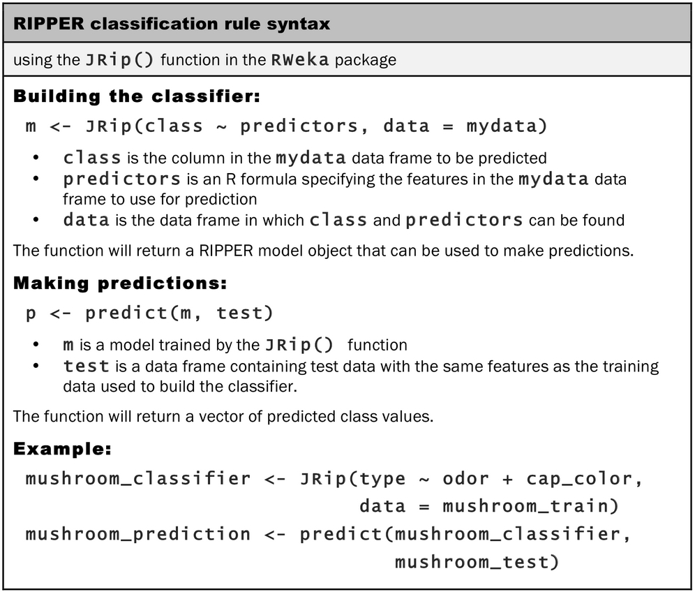
As shown in the syntax box, the process of training a JRip() model is very similar to the training of a OneR() model. This is one of the pleasant benefits of the R formula interface: the syntax is consistent across algorithms, which makes it simple to compare a variety of models.
Let's train the JRip() rule learner as we had done with OneR(), allowing it to find rules among all of the available features:
> mushroom_JRip <- JRip(type ~ ., data = mushrooms)
To examine the rules, type the name of the classifier:
> mushroom_JRip

JRIP rules:
===========
(odor = foul) => type=poisonous (2160.0/0.0)
(gill_size = narrow) and (gill_color = buff)
  => type=poisonous (1152.0/0.0)
(gill_size = narrow) and (odor = pungent)
  => type=poisonous (256.0/0.0)
(odor = creosote) => type=poisonous (192.0/0.0)
(spore_print_color = green) => type=poisonous (72.0/0.0)
(stalk_surface_below_ring = scaly)
  and (stalk_surface_above_ring = silky)
    => type=poisonous (68.0/0.0)
(habitat = leaves) and (gill_attachment = free)
  and (population = clustered)
  => type=poisonous (16.0/0.0)
=> type=edible (4208.0/0.0)

Number of Rules : 8
The JRip() classifier learned a total of eight rules from the mushroom data. An easy way to read these rules is to think of them as a list of if–else statements, similar to programming logic. The first three rules could be expressed as:
Finally, the eighth rule implies that any mushroom sample that was not covered by the preceding seven rules is edible. Following the example of our programming logic, this can be read as:
- Else, the mushroom is edible
The numbers next to each rule indicate the number of instances covered by the rule and a count of misclassified instances. Notably, there were no misclassified mushroom samples using these eight rules. As a result, the number of instances covered by the last rule is exactly equal to the number of edible mushrooms in the data (N = 4,208).
The following figure provides a rough illustration of how the rules are applied to the mushroom data. If you imagine the large oval as containing all mushroom species, the rule learner identified features, or sets of features, which separate homogeneous segments from the larger group. First, the algorithm found a large group of poisonous mushrooms uniquely distinguished by their foul odor. Next, it found smaller and more specific groups of poisonous mushrooms. By identifying covering rules for each of the varieties of poisonous mushrooms, all of the remaining mushrooms were edible. Thanks to Mother Nature, each variety of mushrooms was unique enough that the classifier was able to achieve 100 percent accuracy.

Figure 5.15: A sophisticated rule learning algorithm identified rules to perfectly cover all types of poisonous mushrooms