Copyright © 2010 Elsevier Inc.. All rights reserved.
Introduction
Historical data first manifested itself as the backups and logfiles we kept and hoped to ignore. We hoped to ignore those datasets because if we had to use them, it meant that something had gone wrong, and we had to recover a state of the database prior to when that happened. Later, as data storage and access technology made it possible to manage massively larger volumes of data than ever before, we brought much of that historical data on-line and organized it in two different ways. On the one hand, backups were stacked on top of one another and turned into data warehouses. On the other hand, logfiles were supplemented with foreign keys and turned into data marts.
We don't mean to say that this is how the IT or computer science communities thought of the development and evolution of warehouses and marts, as it was happening over the last two decades. Nor is it how they think of warehouses and marts today. Rather, this is more like what philosophers call a rational reconstruction of what happened. It seems to us that, in fact, warehouses are the form that backup files took when brought on-line and assembled into a single database instance, and data marts are the form that transaction logs took when brought on-line and assembled into their database instances. The former is history as a series of states that things go through as they change over time. The latter is history as a series of those changes themselves.
But warehouses and data marts are macro structures. They are structures of temporal data at the level of databases and their instances. In this book, we are concerned with more micro-level structures, specifically structures at the level of tables and their instances. And at this level, temporal data is still a second-class citizen. To manage it, developers have to build temporal structures and the code to manage them, by hand. In order to fully appreciate both the costs and the benefits of managing temporal data at this level, we need to see it in the context of methods of temporal data management as a whole. In Chapter 1, the context will be historical. In the next chapter, the context will be taxonomic.
In this book, we will not be discussing hardware, operating systems, local and distributed storage networks, or other advances in the platforms on which we construct the places where we keep our data and the pipelines through which we move it from one place to another. Of course, without significant progress in all of these areas, it would not be possible to support the on-line management of temporal data. The reason is that, since the total amount of non-current data we might want to manage on-line is far greater than the total amount of current data that we already do manage on-line, the technologies for managing on-line data could easily be overwhelmed were those technologies not rapidly advancing themselves.
We have already mentioned, in the Preface, the differences between non-temporal and temporal data and, in the latter category, the two ways that time and data are interwoven. However it is not until Part 2 that we will begin to discuss the complexities of bi-temporal data, and how Asserted Versioning renders that complexity manageable. But since there are any number of things we could be talking about under the joint heading of time and data, and since it would be helpful to narrow our focus a little before we get to those chapters, we would like to introduce a simple mental model of this key set of distinctions.
Non-Temporal, Uni-Temporal and Bi-Temporal Data
Figure Part 1.1 is an illustration of a row of data in three different kinds of relational table. 1id is our abbreviation for “unique identifier”, PK for “primary key”, bd1 and ed1 for one pair of columns, one containing the begin date of a time period and the other containing the end date of that time period, and bd2 and ed2 for columns defining a second time period. 2 For the sake of simplicity, we will use tables that have single-column unique identifiers.
1Here, and throughout this book, we use the terminology of relational technology, a terminology understood by data management professionals, rather than the less well-understood terminology of relational theory. Thus, we talk about tables rather than relations, and about rows in those tables rather than tuples.
2This book illustrates the management of temporal data with time periods delimited by dates, although we believe it will be far more common for developers to use timestamps instead. Our use of dates is motivated primarily by the need to display rows of temporal data on a single printed line.
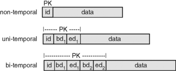 |
| Figure Part 1.1 Non-Temporal, Uni-Temporal and Bi-Temporal Data. |
The first illustration in Figure Part 1.1 is of a non-temporal table. This is the common, garden-variety kind of table that we usually deal with. We will also call it a conventional table. In this non-temporal table, id is the primary key. For our illustrative purposes, all the other data in the table, no matter how many columns it consists of, is represented by the single block labeled “data”.
In a non-temporal table, each row stands for a particular instance of what the table is about. So in a Customer table, for example, each row stands for a particular customer and each customer has a unique value for the customer identifier. As long as the business has the discipline to use a unique identifier value for each customer, the DBMS will faithfully guarantee that the Customer table will never concurrently contain two or more rows for the same customer.
The second illustration in Figure Part 1.1 is of a uni-temporal Customer table. In this kind of table, we may have multiple rows for the same customer. Each such row contains data describing that customer during a specified period of time, the period of time delimited by bd1 and ed1.
In order to keep this example as straightforward as possible, let's agree to refrain from a discussion of whether we should or could add just the period begin date, or just the period end date, to the primary key, or whether we should add both dates. So in the second illustration in Figure Part 1.1, we show both bd1 and ed1 added to the primary key, and in Figure Part 1.2 we show a sample uni-temporal table.
 |
| Figure Part 1.2 A Uni-Temporal Table. |
Following a standard convention we used in the articles leading up to this book, primary key column headings are underlined. For convenience, dates are represented as a month and a year. The two rows for customer id-1 show a history of that customer over the period May 2012 to January 2013. From May to August, the customer's data was 123; from August to January, it was 456.
Now we can have multiple rows for the same customer in our Customer table, and we (and the DBMS) can keep them distinct. Each of these rows is a version of the customer, and the table is now a versioned Customer table. We use this terminology in this book, but generally prefer to add the term “uni-temporal” because the term “uni-temporal” suggests the idea of a single temporal dimension to the data, a single kind of time associated with the data, and this notion of one (or two) temporal dimensions is a useful one to keep in mind. In fact, it may be useful to think of these two temporal dimensions as the X and Y axes of a Cartesian graph, and of each row in a bi-temporal table as represented by a rectangle on that graph.
Now we come to the last of the three illustrations in Figure Part 1.1. Pretty clearly, we can transform the second table into this third table exactly the same way we transformed the first into the second: we can add another pair of dates to the primary key. And just as clearly, we achieve the same effect. Just as the first two date columns allow us to keep multiple rows all having the same identifier, bd2 and ed2 allow us to keep multiple rows all having the same identifier and the same first two dates.
At least, that's the idea. In fact, as we all know, a five-column primary key allows us to keep any number of rows in the table as long as the value in just one column distinguishes that primary key from all others. So, for example, the DBMS would allow us to have multiple rows with the same identifier and with all four dates the same except for, say, the first begin date.
This first example of bi-temporal data shows us several important things. However, it also has the potential to mislead us if we are not careful. So let's try to draw the valid conclusions we can from it, and remind ourselves of what conclusions we should not draw.
First of all, the third illustration in Figure Part 1.1 does show us a valid bi-temporal schema. It is a table whose primary key contains three logical components. The first is a unique identifier of the object which the row represents. In this case, it is a specific customer. The second is a unique identifier of a period of time. That is the period of time during which the object existed with the characteristics which the row ascribes to it, e.g. the period of time during which that particular customer had that specific name and address, that specific customer status, and so on.
The third logical component of the primary key is the pair of dates which define a second time period. This is the period of time during which we believe that the row is correct, that what it says its object is like during that first time period is indeed true. The main reason for introducing this second time period, then, is to handle the occasions on which the data is in fact wrong. For if it is wrong, we now have a way to both retain the error (for auditing or other regulatory purposes, for example) and also replace it with its correction.
Now we can have two rows that have exactly the same identifier, and exactly the same first time period. And our convention will be that, of those two rows, the one whose second time period begins later will be the row providing the correction, and the one with the earlier second time period will be the row being corrected. Figure Part 1.3 shows a sample bi-temporal table containing versions and a correction to one of those versions.
 |
| Figure Part 1.3 A Bi-Temporal Table. |
In the column ed2, the value 9999 represents the highest date the DBMS can represent. For example, with SQL Server, that date is 12/31/9999. As we will explain later, when used in end-date columns, that value represents an unknown end date, and the time period it delimits is interpreted as still current.
The last row in Figure Part 1.3 is a correction to the second row. Because of the date values used, the example assumes that it is currently some time later than March 2013. Until March 2013, this table said that customer id-1 had data 456 from August 2013 to the following January. But beginning on March 2013, the table says that customer id-1 had data 457 during exactly that same period of time.
We can now recreate a report (or run a query) about customers during that period of time that is either an as-was report or an as-is report. The report specifies a date that is between bd2 and ed2. If the specified date is any date from August 2012 to March 2013, it will produce an as-was report. It will show only the first three rows because the specified date does not fall within the second time period for the fourth row in the table. But if the specified date is any date from March 2013 onwards, it will produce an as-is report. That report will show all rows but the second row because it falls within the second time period for those rows, but does not fall within the second time period for the second row.
Both reports will show the continuous history of customer id-1 from May 2012 to January 2013. The first will report that customer id-1 had data 123 and 456 during that period of time. The second will report that customer id-1 had data 123 and 457 during that same period of time. So bd1 and ed1 delimit the time period out in the world during which things were as the data describes them, whereas bd2 and ed2 delimit a time period in the table, the time period during which we claimed that things were as each row of data says they were.
Clearly, with both rows in the table, any query looking for a version of that customer, i.e. a row representing that customer as she was at a particular point or period in time, will have to distinguish the two rows. Any query will have to specify which one is the correct one (or the incorrect one, if that is the intent). And, not to anticipate too much, we may notice that if the end date of the second time period on the incorrect row is set to the same value as the begin date of the second time period on its correcting row, then simply by querying for rows whose second time period contains the current date, we will always be sure to get the correct row for our specific version of our specific customer.
That's a lot of information to derive from Figure Part 1.1Figure Part 1.2 and Figure Part 1.3. But many experienced data modelers and their managers will have constructed and managed structures somewhat like that third row shown in Figure Part 1.1. Also, most computer scientists who have worked on issues connected with bi-temporal data will recognize that row as an example of a bi-temporal data structure.
This illustrates, we think, the simple fact that when good minds think about similar problems, they often come up with similar solutions. Similar solutions, yes; but not identical ones. And here is where we need to be careful not to be misled.
Not to Be Misled
Given the bi-temporal structure shown here, any good IT development team could transform a conventional table into a bi-temporal table of that same general structure. But there is a significant amount of complexity which must then be managed. For example, consider the fact mentioned just above that, with a table like this, the DBMS will permit us to insert a new row which is identical to a row already on the table except for the begin date of the first time period or, for that matter, except for the end date of the first time period. But that would be a mistake, a mistake that would allow “overlapping versions” into the table.
Once again, experienced data management professionals may be one step ahead of us. They may already have recognized the potential for this kind of mistake in the kind of primary key that the third table illustrates, and so what we have just pointed out will not be news to them.
But that mistake, the “overlapping versions” mistake, is just one thing a development group will have to write code to prevent. There is an entire web of constraints, beyond those the DBMS can enforce for us, which determine when inserts, updates and deletes to uni-temporal or bi-temporal tables are and are not valid. For example, think of the possibilities of getting it wrong when it comes to a delete cascade that begins with, or comes to as it cascades, a row in a temporal table; or with referential integrity dependencies in which the related rows are temporal. Or the possibilities of writing queries that have to correctly specify three logical components to select the one row the query author is interested in, two of those components being time periods that may or may not intersect in various ways. Continuing on, consider the possibilities involved in joining bi-temporal tables to one another, or to uni-temporal tables, or to non-temporal tables!
This is where computer science gets put to good use. By now, after more than a quarter-century of research, academics are likely to have identified most of the complex issues involved in managing temporal data, even if they haven't come to an agreement on how to deal with all of them. And given the way they think and write, they are likely to have described these issues, albeit in their own mathematical dialects, at a level of detail from which we IT professionals can both design and code with confidence that further bi-temporal complexities probably do not lie hidden in the bushes.
So one reason IT practitioners should not look at Figure Part 1.1Figure Part 1.2 and Figure Part 1.3 and conclude that there is nothing new here is that there is a great deal more to managing temporal data than just writing the DDL for temporal schemas. And if many practitioners remain ignorant of these complexities, it is probably because they have never made full use of the entire range of uni-temporal functionality, let alone of bi-temporal functionality. In fact, in our experience, which between us amounts to over a half-century of IT consulting, for dozens of clients, we have seen little in the way of temporal data management beyond a limited use of the capabilities of uni-temporal versioned tables.
So for most of us, there is a good deal more to learn about managing temporal data. Most of the code that many of us have written to make sure that uni- or bi-temporal updates are done correctly addresses only the tip of the iceberg of temporal data management complexities.
Glossary References
Glossary entries whose definitions form strong interdependencies are grouped together in the following list. The same Glossary entries may be grouped together in different ways at the end of different chapters, each grouping reflecting the semantic perspective of each chapter. There will usually be several other, and often many other, Glossary entries that are not included in the list, and we recommend that the Glossary be consulted whenever an unfamiliar term is encountered.
9999
time period
historical data
non-temporal data
uni-temporal data
object
version
..................Content has been hidden....................
You can't read the all page of ebook, please click here login for view all page.