13. Re-Presenting Internalized Pipeline Datasets
Contents
Internalized Pipeline Datasets292
Pipeline Datasets as Queryable Objects296
Posted History: Past Claims About the Past297
Posted Updates: Past Claims About the Present298
Posted Projections: Past Claims About the Future299
Current History: Current Claims About the Past300
Current Data: Current Claims About the Present301
Current Projections: Current Claims About the Future303
Pending History: Future Claims About the Past304
Pending Updates: Future Claims About the Present305
Pending Projections: Future Claims About the Future306
Mirror Images of the Nine-Fold Way307
The Value of Internalizing Pipeline Datasets308
Glossary References309
In Chapter 12, we introduced the concept of pipeline datasets. These are files, tables or other physical datasets in which the managed object itself represents a type and contains multiple managed objects each of which represents an instance of that type, and which in turn themselves contain instances of other types. Using the language of tables, rows and columns, these managed objects are tables, the instances they contain are rows, and those last-mentioned types are the columns of those tables, whose instances describe the properties and relationships of the objects represented by those rows.
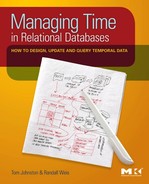
Because our focus is temporal data management at the level of tables and rows, and not at the level of databases, we have discussed pipeline datasets as though there were a distinct set of them for each production table. Figure 13.1 shows one conventional table, and a set of eight pipeline datasets related to it.
 |
| Figure 13.1 Physically Distinct Pipeline Datasets. |
What Figure 13.1 illustrates is a simplification of the always complex and usually messy physical database environment which IT departments everywhere must manage. Pipeline datasets may often contain data targeted at, or derived from, several tables within that database. They do not necessarily target, or derive from, single tables within a database. In addition, the IT industry has only the broadest of categories of pipeline datasets, categories such as batch transaction tables, logfiles of processed transactions, history tables, or staging areas where unusually complicated data transformations are carried out before the data is moved back into the production tables from whence it originated.
Figure 13.1 shows eight different types of pipeline datasets surrounding a conventional table of current data. These nine datasets align with the set of nine categories of temporal data which we introduced in Chapter 12.
Given a bi-temporal framework of two temporal dimensions, in each of which data can exist in the past, the present or the future, this set of nine categories is what results from the intersection of those two temporal dimensions. In addition, since the past, present and future are clear and distinct within each temporal dimension, and since each dimension is clear and distinct from the other, the result of this intersection is a set of nine categories which are themselves clear and distinct, which are, precisely, jointly exhaustive and mutually exclusive. Like our taxonomies, they cover all the ground there is to cover, and they don't overlap. Like our taxonomies, they are what mathematicians call a partitioning of their domain. Like our taxonomies, they assure us that in our discussions, we won't overlook anything and we won't confuse anything with anything else.
In the previous chapter, we showed how to physically internalize one particular kind of pipeline dataset within the production tables which are their destinations or points of origin. We showed how to turn them from distinct physical collections of data into logical collections of data that share residence in a single physical table.
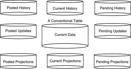
The internalization of pipeline datasets is illustrated in Figure 13.2. These internalizations of pipeline datasets are not themselves managed objects to either the operating system or the DBMS. They are managed objects only to the AVF. The operating system recognizes and manages database instances, but is neither aware of nor can manage tables, rows, columns or the other managed objects that exist within database instances. As for the DBMS, once these pipeline datasets are internalized, all it sees is the production table itself, and the columns and rows of that table.
 |
| Figure 13.2 Internalized Pipeline Datasets. |
In this chapter, we show how to re-present these internalized datasets as queryable objects. We use the hyphenated form “re-present” advisedly. We do mean that we will show how to represent those internalized datasets as queryable objects, in the ordinary sense of the word “represent”. But we also wish to emphasize that we are re-presenting, i.e. presenting again, things whose presence we had removed. 1 Those things are the physical pipeline datasets which, in the previous chapter, we showed how to internalize within the production tables which are their destinations or points of origin.
1We also wish to avoid confusion with our technical term represent, in which an object, we say, is represented in an effective time clock tick within an assertion time clock tick just in case business data describing that object exists on an asserted version row whose assertion and effective time periods contain those clock tick pairs.
For example, we show how to provide, as queryable objects, all the pending transactions against a production table, or a logfile of posted transactions that have already been applied to that table, or a set of data from that table which we currently claim to be true, or that same set of data but as it was originally entered and prior to any corrections that may have been made to it.
We do not claim that any of these eight types of pipeline dataset correspond to data that supports a specific business need. For the most part, that will not be the case. For example, auditors will frequently want to look at Posted History pipeline datasets, i.e. at the rows that belong to that logical category of temporal data. But they will usually want to see current assertions about the historical past of the objects they are interested in, along with those past assertions. The current assertions about historical data are logically part of, as we will see, the Posted Updates pipeline dataset. So to provide queryable objects corresponding to their specific business requirements, auditors will usually write queries directly against asserted version tables, queries that combine and filter data from any number of these pipeline datasets.
To take another example, the Pending Projections pipeline dataset does not distinguish data in the near assertion time future from data in the far assertion time future. Yet deferred assertions with an assertion begin date that will become current an hour from now serve an entirely different business purpose than deferred assertions whose assertion begin date is January 1st, 5000. So to provide queryable objects corresponding to real business requirements, we will often have to write queries that filter out rows from within a single pipeline dataset, and combine rows from multiple pipeline datasets.
Internalized Pipeline Datasets
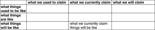
We can say what things used to be like, what they are like, and also what they will be like. These statements we can make are statements about, respectively, the past, the present and the future. In a table in a database, each row makes one such statement. In conventional tables, however, the only rows are ones that make statements about the present.
These things we say represent what we claim is true. Of course, as we saw in Chapter 12, we can equally well say that they represent what we accept as true, agree is true, assent to or assert as true, or believe, know or think is true. For now, we'll just call them our truth claims, or simply our claims, about the statements made by rows in our tables.
Besides what we currently claim is true, there are also claims that we once made but are no longer willing to make. These are statements that, based on our current understanding of things, are not true, or should no longer be considered as reliable sources of information. It is also the case that we may have statements—whether about the past, the present or the future—that we are not yet willing to claim are true, but which nonetheless are “works in progress” that we intend to complete and that, at that time, we will be willing to claim are true. Or perhaps they are complete, and we are pretty certain that they are correct, but we are waiting on a business decision-maker to review them and approve them for release as current assertions. The former is a set of transactions about to be applied to the database. The latter is a set of data in a staging area, either waiting for additional work to be performed on it, or waiting for review and approval.
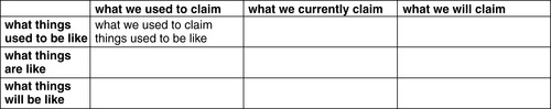
So if statements may be about what things were, are or will be like, and claims about statements may have once been made and later repudiated, or be current claims, or be claims that we are not yet willing to make but might at some time in the future be willing to make, then the intersection of facts and claims creates a matrix of nine temporal combinations. That matrix is shown in Figure 13.3. 2
2With the substitution of the word “claims” for “beliefs”, this is the same matrix shown in Figure 12.1. Chapter 12 also contains a discussion of the interchangeability of “claims”, “beliefs” and several other terms. We note, however, that “claims” is a stronger word than “beliefs” in this sense, that some of the things we believe are true are things we are nonetheless not yet willing to claim are true. We take “claims”, and “asserts” or “assertions”, to be synonymous, and the other equivalent terms discussed in Chapter 12 to be terminological variations that appear more or less suitable in different contexts.
 |
| Figure 13.3 Facts, Claims and Time. |
The reason we are interested in the intersection of facts and claims is that rows in database tables are both. All rows in database tables represent factual claims. One aspect of the row is that it represents a statement of fact. The other aspect is that it represents a claim that that statement of fact is, in fact, true. This is just as true of conventional tables as it is of asserted version tables.
When dealing with periods of time, as we are, the past includes all and only those periods of time which end before Now(). The future includes all and only those periods of time which begin after Now(). The present includes all and only those periods of time which include Now().
Every row in a bi-temporal table is tagged with two periods of time, which we call assertion time and effective time. Consequently, every row falls into one of these nine categories. Conventional tables contain rows which exist in only one of these nine temporal combinations. They are rows which represent current claims about what things are currently like. But since conventional tables do not contain any of the other eight categories of rows, their rows don't need explicit time periods to distinguish them from rows in those other categories. And in conventional tables, of course, they don't have them.
Both the assertion and the effective time periods of conventional rows are co-extensive with their physical presence in their tables. They begin to be asserted, and also go into effect, when they are created; and they remain asserted, and also remain in effect, until they are deleted. They don't keep track of history because they aren't interested in it. They don't distinguish updates which correct mistakes in data from updates which keep data current with a changing reality, ultimately because the business doesn't notice the difference, or is willing to tolerate the ambiguity in the data.
So conventional tables, all in all, are a poor kind of thing. They do less than they could, and less than the business needs them to do. They overwrite history. They don't distinguish between correcting mistakes and making changes to keep up with a changing world. And these conventional tables, as we all know, make up the vast majority of all persistent object tables managed by IT departments.
We put up with tables like these because the IT profession isn't yet aware that there is an alternative and because, by dint of hard work, we can make up for the shortcomings of these tables. Data which falls into one of the other eight categories can usually be found somewhere, or reconstructed from data that can be found somewhere. If all else fails, DBMS archives and backups, and their associated transaction logs, will usually enable us to recreate any state that the database has been in. They will allow us to re-present six of the nine temporal categories we have identified. 3
3That's the idea, anyway. In reality, this “data of last resort” isn't always there when we go looking for it. Backups and logfiles are rarely kept forever, so the data we need may have been purged or written over. There will inevitably be occasional intervals during which the system hiccupped, and simply failed to capture the data in the first place. If the data is still available, it might not be in a readily accessible format because of schema changes made after it was captured.
The three categories that cannot be re-presented from backups and logfiles are the three categories of future claims—things we are going to make our databases say (unless we change our minds) about what things once were like, or are like now, or may be like in the future. Future claims often start out as scribbled notes on someone's desk. But once inside the machine, they exist in transaction datasets, in collections of data that are intended, at some time or other, to be applied to the database and become currently asserted data.
In the previous chapter, we called the eight categories of data which are not current claims about the present, pipeline datasets, collections of data that exist at various points along the pipelines leading into production tables or leading out from them. As physically separate from those production tables, these collections of data are generally not immediately available for business use. Usually, IT technical personnel must do some work on these physical files or tables before a business user can query them for information.
This takes time, and until the work is complete, the information is not available. By the time the work is complete, the business value of the information may be much reduced. This work also has its costs in terms of how much time those technicians must spend to prepare that data to be queried. In addition, even without special requests for information in them, these physical datasets, taken together, constitute a significant management cost for IT.
With multiple points of rest in the pipelines leading into and out of production database tables, there are multiple points at which data can be lost. For example, data can be accidentally deleted before any copies are made. For datasets in the inflow pipelines, and which have not yet made it into the database itself, the only recourse for lost data is to reacquire or recreate the data. If prior datasets in the pipeline have already been legitimately deleted (legitimately because the data had successfully made it to the next downstream point), then we may have to go all the way back to the original point at which the data was first acquired or created. This can impose significant delays in getting the data to its consumers, and significant costs in reacquiring or recreating it and in moving it, for a second time, down the pipeline. And this risk is quite real because, prior to making it into the database, the backups and logfiles which protect data once it has reached the DBMS are not yet available.
By internalizing these datasets within the production tables whose data they contain, we eliminate the costs of managing them, including the costs of recovering from mistakes made in managing them. We now turn to the task of re-presenting what were physically distinct managed objects, external to production tables. We re-present them as queryable objects, showing how queries can produce result sets containing exactly the data that would have been in those physical datasets, had we not internalized them.
Pipeline Datasets as Queryable Objects
We emphasize once more that most business queries for temporal data will not focus on data from a single one of these eight internalized pipeline datasets. Together with currently asserted current data, these eight other categories of temporal data constitute a partitioning of all bi-temporal data. Like the Allen relationship queries we will discuss in the next chapter, we focus on these queries in spite of the fact that they are not real-world business queries. We focus on them because, as a set, they are guaranteed to be complete. If these eight categories of pipeline datasets can be internalized, then we can be certain that any real-world business dataset—one destined to update a production table, or one derived from a production table—can also be internalized. In the next chapter, once we have seen that any Allen relationship against asserted version data can be expressed in a query, we will be similarly certain that any query whatsoever can be expressed against asserted version tables.
In each case, we will illustrate these queries in the context of CREATE VIEW statements. From the point of view of the semantics involved, there is no difference between direct queries and SQL VIEW statements. But actual VIEW statements lend a little more substance to the notion of re-presenting internalized pipeline datasets as queryable objects.
Posted History: Past Claims About the Past
The Posted History dataset consists of all those rows in an asserted version table which lie in both the assertion time past and also in the effective time past. Its subject matter is things as they used to be. Its rows are claims about what is now part of history which we are no longer willing to make. Posted History is a record of all the times we got it wrong about what is now the past, up to but not including our current claims about that past. Those current claims, of course, are the ones in which we finally, we hope, got it right.
Here is the view which re-presents Posted History. With the suffix “Post_Hist” standing for “posted history”, it looks like this:
CREATE VIEW V_Policy_Post_Hist
AS SELECT oid, asr_beg_dt, asr_end_dt, eff_beg_dt, eff_end_dt,
client, type, copay
FROM Policy_AV
WHERE asr_end_dt <= Now()
AND eff_end_dt <= Now()
Note that Posted History is a bi-temporal collection of data. Neither temporal dimension is restricted to a point in time, and so both time periods must be included on all rows in the view. The unique identifier for this or for any other bi-temporal view of an asserted version table, is the combination of oid, assertion time period and effective time period.
 |
| Figure 13.4. |
| Posted History. |
Because Asserted Versioning manages the two pairs of dates as PERIOD datatypes, either or both can be used to represent the time period. So, in an asserted version table and, therefore, in any bi-temporal view based on it, any of the following are unique identifiers: {oid + asr-beg + eff-beg}, {oid + asr-end + eff-beg}, {oid + asr-beg + eff-end}, or {oid + asr-end + eff-end}. In addition, the identifiers will remain unique even if we add either one or two more dates from the date pairs to them. For example, {oid + asr-beg + eff-beg + eff-end} is also unique. This is important to know when creating indexes for performance, as described in Chapter 15.
Any report about the effective-time past can be either an as-was or an as-is report. If it is an as-is report, it can be produced from Current History. But if it is an as-was report, it can be produced only from Posted History.
Posted Updates: Past Claims About the Present
The Posted Updates dataset consists of all those rows in an asserted version table which lie in the assertion time past but in the effective time present. Its subject matter is things as they currently are. Its rows are claims about these things which we are no longer willing to make. Posted Updates are a record of all the times we got it wrong about what is now the present, up to but not including our current claims about that present. Those current claims, of course, are the ones in which we finally, we hope, got it right.
Here is the view which re-presents Posted Updates. With the suffix “Post_Upd” standing for “posted updates”, it looks like this:
CREATE VIEW V_Policy_Post_Upd
AS SELECT oid, asr_beg_dt, asr_end_dt, eff_beg_dt, eff_end_dt,
client, type, copay
FROM Policy_AV
WHERE asr_end_dt <= Now()
AND eff_beg_dt <= Now() AND eff_end_dt > Now()
The Posted Updates dataset is also a bi-temporal collection of data, and so both time periods must be included on all rows in the view. The unique identifier for this or for any other bi-temporal view of an asserted version table, is the combination of oid, any one or both of the assertion dates, and any one or both of the effective dates.
 |
| Figure 13.5. |
| Posted Updates. |
Posted Projections: Past Claims About the Future
The Posted Projections dataset consists of all those rows in an asserted version table which lie in the assertion time past but in the effective time future. Its subject matter is things as they might have turned out to be. Its rows are claims about these things which we are no longer willing to make. Posted Projections are a record of all the times we got it wrong about what currently lies in the future, up to but not including our current claims about that future. Those current claims, of course, are the ones in which we finally, we hope, got it right.
Here is the view which re-presents Posted Projections. With the suffix “Post_Proj” standing for “posted projections”, it looks like this:
CREATE VIEW V_Policy_Post_Proj
AS SELECT oid, asr_beg_dt, asr_end_dt, eff_beg_dt, eff_end_dt,
client, type, copay
FROM Policy_AV
WHERE asr_end_dt <= Now()
AND eff_beg_dt > Now()
The Posted Projections dataset is also a bi-temporal collection of data, and so both time periods must be included on all rows in the view. The unique identifier for this or for any other bi-temporal view of an asserted version table, is the combination of oid, any one or both of the assertion dates, and any one or both of the effective dates.
The rows in this view are mistakes which never became effective. In a more sinister light, they are forecasts which never came true, and which those making them perhaps knew or suspected would never come true. Note, however, that we can certainly be held responsible for statements about what never came to be. We can be held responsible for a statement made by any row that has ever existed in current assertion time. In this case, these rows were once asserted. Once upon a time, they were claims made about what the future will be like. Bernie Madoff is in jail for making such claims.
 |
| Figure 13.6. |
| Posted Projections. |
Of course, we can always be mistaken about what the future will be like. But that's not the point about responsibility. The point is that we made those claims. Due allowance will be made for the fact that they were claims about the future.
If they turn out to be false, that doesn't necessarily mean that we intended to mislead others. In making those claims, we may have taken all due diligence, and simply have made a responsible but mistaken projection. On the other hand, we may have been irresponsible, we may not have taken due diligence. On the basis of nothing more than a hunch, we may have presented to the world, as actionable projections responsibly made, statements about what we merely guessed the future might be like.
So assertions are not just claims that statements are true, although that is an often convenient shorthand for saying what assertions are. More precisely, assertions are claims that statements are not only true, but are also actionable, that they are good enough for their intended uses. And since statements about the future are neither true nor false, at the time they are made, the best that we can assert about them is that they are responsibly made, and are therefore actionable.
Current History: Current Claims About the Past
The Current History dataset consists of all those rows in asserted version tables which lie in the assertion time present but in the effective time past. Its subject matter is things as they used to be. Its rows are current claims about what is now the past. Current History is a record of what we currently believe things used to be like.
Here is the view which re-presents Current History. With the suffix “Curr_Hist” standing for “current history”, it looks like this:
CREATE VIEW V_Policy_Curr_Hist
AS SELECT oid, eff_beg_dt, eff_end_dt, client, type, copay
FROM Policy_AV
WHERE asr_beg_dt <= Now() AND asr_end_dt > Now()
AND eff_end_dt <= Now()
 |
| Figure 13.7. |
| Current History. |
The Current History dataset is a uni-temporal collection of data. It re-presents, as a queryable object, what is usually called a history table, a table of all versions of objects, up to but not including the current version.
Because there cannot be two current assertions about the same object during the same or overlapping periods of effective time, assertion time is not needed in this view. All the rows in this dataset are currently asserted rows. And so only one time period is part of this view. The unique identifier of the data in the view is {oid + eff-beg + eff-end}. In fact, with just either one of those two dates, it is still a unique identifier.
In history tables as they are currently used in IT, assertion time differences are not recorded. Some history tables will be as-was tables, i.e. tables in which each row remains exactly as it was when it became history. Others will be as-is tables, i.e. tables in which errors in the history table data are corrected as they are discovered, but corrected by means of overwriting the original data. In yet other cases, there is no explicit policy defining the history table as an as-is or an as-was table; and so if we use the history table, for example, to recreate a report as it was originally run, we will probably produce a report with a mixture of data as originally entered, together with other data that has been corrected, with no way to tell which is which.
Asserted Versioning supports both kinds of history. The Posted History dataset is equivalent to an as-was history table. The Current History dataset is equivalent to an as-is history table, a table which tells us what we currently believe the past to have been like. As such, it is a currently asserted version table. So if it is used to rerun reports as of some point in past effective time, those reports will reflect all corrections made to that data since that time.
Queries supporting specific business requests for information can, of course, be written against these internalizations of pipeline datasets. For example, if we are interested only in 2009's historical data, as we currently claim that data to be, we can issue a query against this view which selects just that data. That query looks like this:
SELECT oid, eff_beg_dt, eff_end_dt, client, type, copay
FROM Policy_V_Curr_Hist
WHERE eff-beg >= 01/01/2009 AND eff_end_dt < 01/01/2010
Current Data: Current Claims About the Present
The Current Data dataset consists of all those rows in an asserted version table which lie in the assertion time present and also in the effective time present. Its subject matter is things as they are now. Its rows are claims about these things which we currently make. Current Data is what most of our database tables contain. It is a record of what we currently believe things are currently like.
If our asserted version table previously existed as a conventional table, there are likely to be any number of production queries that reference it. To make the conversion of this table to an asserted version table transparent to these queries, we must rename the table and use its original name as the name of this view. This is why we have renamed such tables by appending “_AV” to them. Doing this for the Policy table we are using in these examples, we renamed it as Policy_AV.
Here is a view preliminary to the one which does re-present Current Data. This view contains all currently asserted current versions.
CREATE VIEW Policy_CACV
AS SELECT oid, client, type, copay
FROM Policy_AV
WHERE asr_beg_dt <= Now() AND asr_end_dt > Now()
AND eff_beg_dt <= Now() AND eff_end_dt > Now()
In the original non-temporal table, there was one row per object. Since each oid uniquely identifies an object, and since there can only be one row for each object that is currently asserted as being currently in effect, this view also contains one row per object. In addition, since, at every point in time, the original table contains rows that represent what we currently believe the objects described by those rows are currently like, an asserted version table of currently asserted current versions will contain, moment for moment, exactly the same business data.
 |
| Figure 13.8. |
| Current Data. |
Like the conventional Policy row, this view uses exactly one row to re-present one policy. But unlike the conventional Policy table, these rows include oids, not the column or columns that were the primary key in the original conventional table. And they include temporal foreign keys, not the column or columns that were the foreign keys in the original table.
So we do not yet have a view which re-presents the original conventional table. The Current Data dataset is row-to-row equivalent to the original table in terms of its contents, but not in terms of its schema. We do not yet have a view to which all queries against the original table can be redirected. That view must replace the oid in Policy_CACV with the original primary key, and replace the TFK with the original foreign key. And it must have the same name as the original table. Here is that view:
CREATE VIEW Policy
AS SELECT policy_nbr AS P.policy_nbr, policy_type AS P.policy_type,
copay_amt AS P.copay_amt, client_nbr AS C.client_nbr
FROM Policy_CACV P
JOIN Client C
ON C.client_oid = P.client_oid
The most frequently used view of any asserted version table is likely to be this current data view. These are precisely those rows that make up the complete contents of a conventional non-temporal table.
Current Projections: Current Claims About the Future
The Current Projections dataset consists of all those rows in an asserted version table which lie in the assertion time present but in the effective time future. Its subject matter is things as they may turn out to be. Its rows are claims about these things which we currently make. Current Projections are a record of what we currently believe things are going to be like; and, of course, we shouldn't make such claims unless we are pretty sure that's how they will turn out to be. If we aren't pretty sure about them, then we should make them, if we make them at all, as pending projections.
 |
| Figure 13.9. |
| Current Projections. |
Here is the view which re-presents Current Projections. With the suffix “Curr_Proj” standing for “current projections”, it looks like this:
CREATE VIEW V_Policy_Curr_Proj
AS SELECT oid, eff_beg_dt, eff_end_dt, client, type, copay
FROM Policy_AV
WHERE asr_beg_dt <= Now() AND asr_end_dt > Now()
AND eff_beg_dt > Now()
As we can see, effective time is explicitly represented in this view, and so the view is a collection of uni-temporal versioned data. As such, it has the unique identifier that all version tables have—{oid + eff-beg+ eff-end}, in which the two dates are not merely two dates, but each the semantically complete representative of a PERIOD datatype.
The Current Projections dataset is the collection of all future versions in an asserted version table that we currently assert as making actionable statements. A simple example of a current projection is a version that shows a change in a policy's copay amount that will go into effect next month. The version exists in current assertion time but in future effective time.
Pending History: Future Claims About the Past
The Pending History dataset consists of all those rows in an asserted version table which lie in the assertion time future but in the effective time past. Its subject matter is things as they used to be. Its rows are claims which we are not yet willing to make about what is now part of history. Pending History is a record of what we may eventually be willing to say the past was like, once we've got all our facts straight.
 |
| Figure 13.10. |
| Pending History. |
Here is the view which re-presents Pending History. With the suffix “Pend_Hist” standing for “pending history”, it looks like this:
CREATE VIEW V_Policy_Pend_Hist
AS SELECT oid, asr_beg_dt, asr_end_dt, eff_beg_dt, eff_end_dt,
client, type, copay
FROM Policy_AV
WHERE asr_beg_dt > Now()
AND eff_end_dt <= Now()
Pending History is history as it will look once we get around to correcting it. One reason we might have pending history is that we have some information about what is needed to correct the past, but not all the information we need. Once that deferred assertion about the past is complete, we can then apply it. Another reason we might have pending history is that we have one or more corrections to the past, but those corrections can't be released until they are approved. Once approval is given, we can apply them, and those deferred assertions about the past will become current assertions about the past.
Pending Updates: Future Claims About the Present
The Pending Updates dataset consists of all those rows in an asserted version table which lie in the assertion time future but in the effective time present. Its subject matter is things as they currently are. Its rows are claims about these things which we are not yet willing to make. The Pending Updates dataset is a record of what we may eventually (or soon) be willing to say things are like right now.
Here is the view which re-presents Pending Updates. With the suffix “Pend_Upd” standing for “pending updates”, it looks like this:
CREATE VIEW Policy_Pend_Upd
AS SELECT oid, asr_beg_dt, asr_end_dt, eff_beg_dt, eff_end_dt, client, type, copay
FROM Policy_AV
WHERE asr_beg_dt > Now()
AND eff_beg_dt <= Now() AND eff_end_dt > Now()
 |
| Figure 13.11. |
| Pending Updates. |
Pending Updates exist in what we called, in the previous chapter, either the assertion-time near future or the assertion-time far future. Those in the near future have an assertion begin date close enough to Now() that the business is willing to let the passage of time make them current. Near future deferred assertions would typically have a begin date that will become current in the next few seconds, hours, days or weeks. In a conventional database, pending updates are transactions accumulated in an external batch transaction file, or perhaps in a batch transaction table within the database.
Far future deferred assertions are the internalization of data located in what are often called staging areas. They are collections of data that are usually more complicated than usual to update. By placing them in far future assertion time, we guarantee that they will not inadvertently become current assertions simply because of the passage of time. They can become current assertions only when, presumably after a review-and-approve process, the business releases them into near-future assertion time.
Pending Projections: Future Claims About the Future
The Pending Projections dataset consists of all those rows in an asserted version table which lie in both the assertion time future and in the effective time future. Its subject matter is things as they may turn out to be. Its rows are claims about what currently lies in the future, but claims which we are not yet willing to make. Pending Projections are a record of what we may eventually be willing to say things are going to be like.
 |
| Figure 13.12. |
| Pending Projections. |
Here is the view which re-presents Pending Projections. With the suffix “Pend_Proj” standing for “pending projections”, it looks like this:
CREATE VIEW Policy_Pend_Proj
AS SELECT oid, asr_beg_dt, asr_end_dt, eff_beg_dt, eff_end_dt, client, type, copay
FROM Policy_AV
WHERE asr_beg_dt > Now()
AND eff_beg_dt > Now()
As we have seen with our other re-presented pipeline datasets, Pending Projections include both the assertion and effective time period as part of the unique identifier because both temporal dimensions are specified as ranges, and neither as points in time.
Mirror Images of the Nine-Fold Way
As we said in Chapter 9, effective time exists within assertion time. First, logically speaking, we make a statement about how things are. Next, logically speaking, we make a truth claim about that statement.
Most of our queries against bi-temporal tables will specify a point in assertion time—most commonly Now()—and then ask for rows asserted at that point in time that were in effect at some point or period of effective time. For example, we might ask for all policies that were in effect on August 23, 2008, as we currently believe them to have been. Or we might ask for all policies which we currently claim were in effect any time in the first half of 2008.
Pinning down a point in assertion time, and then asking for versions of objects claimed at that point in time to be correct, is the general form that queries will take when posed by business users. But we can look at bi-temporal data from the opposite point of view as well. We can pin down a point or period in effective time, and ask for everything we ever asserted about things at that point in time.
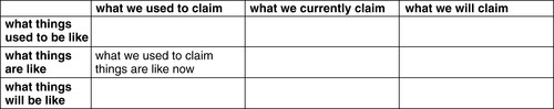
It would not be too misleading to call this the auditor's point of view. From this point of view, we are interested in the history of our claims about what is true, not in the history of what actually happened out there in the world. Of course, we could also ask for all future assertions about a given point in effective time. But auditors, by the nature of their work, have little interest in future assertions. By the same token, they are very interested in past assertions, along with current ones. So an auditor's mirror-image of the nine categories reduces to a set of six categories, those shown in Figure 13.13.
 |
| Figure 13.13 The Auditor's Mirror Image of the Nine-Fold Way. |
These views that auditors are interested in are physically the same ones we have already described. The “mirror-image” is in perspective, not in content.
The Value of Internalizing Pipeline Datasets
The cost of managing physical pipeline datasets is high. This cost is seldom discussed because it is universally thought to be just an inevitable cost of doing business. Bringing down this cost is a matter of doing all those various things that IT management has done for decades, and continues to do. Quality control procedures are put in place so errors don't creep into our databases and later have to be backed out. The platform costs of storing, transforming, and moving data into and out of pipeline datasets are controlled by minimizing redundancy, and by moving datasets up and down the storage hierarchy. Software that sets up and runs production schedules minimizes the human costs of scheduling work involving these pipeline datasets.
But the work of managing pipeline datasets is tedious. And whenever the management of these datasets is a one-off kind of thing, i.e. whenever the development group has to manage these datasets rather than the IT Operations group that handles scheduled maintenance, errors in managing them are not uncommon.
Asserted Versioning does not offer a way to more efficiently manage pipeline datasets. It offers a way to eliminate them and, consequently, eliminate the totality of their management costs! There will always be some circumstances in which data must be manipulated in external pipeline datasets. But these can become the exception rather than the rule.
In place of these pipeline datasets, Asserted Versioning stores the information contained in those pipeline datasets internally, within the production tables that are their sources and destinations. Pending transactions can be stored within the production tables themselves. Posted transactions can be, too. Data staging areas can also exist as semantically distinct sets of rows, physically contained within production tables. Pipeline datasets, then, cease to exist as distinct physical objects. They become virtualized, as semantically distinct collections of rows all physically existing within the same tables, re-presented in different views.
We may think that the principal cost elimination benefit of internalizing pipeline datasets is that it reduces the number of distinct datasets that programs, SQL and production scheduling software have to identify and manage. This is a reduction in the cost of the mechanics of pipeline datasets. Instead of assembling data from multiple tables, it already exists all in one place.
But the more significant cost reduction has to do with the semantics of pipeline datasets. With all data about the same things in the same place, we will, all of us, find all of it when we go looking for it. The most junior member of the business community will find the same set of data for his queries that the most senior member does. There won't be differences in completeness of the source data, or quality of that data, as there so often are in today's business world and today's collections of business data.
When we need any of this data, we won't have to go looking for it. All of the data about what we once thought was true, or what we currently think is true, or what we are not yet willing to assert is true, will be available by simply changing the assertion point-in-time selection criterion on views and queries. By changing that predicate in a WHERE clause to a past point in assertion time, we will be able to access the internalized re-presentation of posted transactions. By changing the predicate to a future point in time, we will be able to access the internalized re-presentation of pending transactions.
By the same token, we will be able to access historical data about what things used to be like from the same table that contains data about what they are like right now, and that may also contain data about what those things are going to be like sometime in the future. Again, it will be as easy as changing a predicate in a WHERE clause.
Glossary References
Glossary entries whose definitions form strong inter-dependencies are grouped together in the following list. The same glossary entries may be grouped together in different ways at the end of different chapters, each grouping reflecting the semantic perspective of each chapter. There will usually be several other, and often many other, glossary entries that are not included in the list, and we recommend that the Glossary be consulted whenever an unfamiliar term is encountered.
We note, in particular, that none of the nine types of pipeline dataset are included in this list. In general, we leave category sets out of these lists, but recommend that the reader look them up in the Glossary.
as-is
as-was
Asserted Versioning Framework (AVF)
assertion time
statement
conventional table
non-temporal table
deferred assertion
far future assertion time
near future assertion time
instance
type
managed object
object
oid
queryable object
pipeline dataset
inflow pipeline
outflow pipeline
internalization of pipeline datasets
re-presentation of pipeline datasets
production database
production table
temporal dimension
temporal transaction
version
..................Content has been hidden....................
You can't read the all page of ebook, please click here login for view all page.