15. Optimizing Asserted Versioning Databases
One concern about Asserted Versioning is with how well it will perform. We believe that with recent improvements in technology, and with the use of the physical design techniques described in this chapter, Asserted Versioning databases can achieve performance very close to that of conventional databases. This is especially true for queries, which are usually the most frequent kind of access to any relational database. The AVF, our own implementation of Asserted Versioning, is designed to operate well with large data volume databases supporting a high volume of mixed-type data retrieval requests.
Bi-Temporal, Conventional, and Non-Temporal Databases
In this section, we compare data volumes and response times in bi-temporal and in conventional databases. We find that differences in both data volumes and response times are generally quite small, and are usually not good reasons for hesitating to implement bi-temporal data in even the largest databases of the world's largest corporations.
Data Volumes in Bi-Temporal and in Conventional Databases
It might seem that a bi-temporal database will have a lot more data in it than a conventional database, and will consequently take a lot longer to process. It is true that the size of a bi-temporal database will be larger than that of an otherwise identical database which contains only current data about persistent objects. But in our consulting engagements, which span several decades and dozens of clients, we have found that in most mission-critical systems, temporal data is jury-rigged into ostensibly non-temporal databases.
There are any number of ways that this may happen. For example, in some systems a version date is added to the primary key of selected tables. In other systems, more advanced forms of best practice versioning (as described in Chapter 4) are employed. Sometimes, history will be captured by triggering an insert into a history table every time a particular non-temporal table is modified. Another approach is to generate a series of periodic snapshot tables that capture the state of a non-temporal table at regular intervals.
Of course, a database with no temporal data at all will certainly be smaller than the same database with temporal data. But adding up the overhead associated with embedded best practice versioning, or with triggered history, periodic snapshots or some combination of these and other techniques, the amount of data in a so-called non-temporal database may be as much or even more than the amount of data in a bi-temporal database.
Throughout this book, we have been using the terms “non-temporal database” and “conventional database” as equivalent expressions. But now we have a reason to distinguish them. From now on, we will call a database “non-temporal” only if it contains no temporal data about persistent objects at all. 1 And from now on, we will use the term “conventional database” to refer to databases that may or may not contain temporal data about persistent objects (and that usually do), but that do not contain explicitly bi-temporal tables and instead incorporate temporal data by using variations on one or more of the ad hoc methods we have described.
1The point of adding “about persistent objects”, of course, is to distinguish between objects and events, as we did in our taxonomy in Chapter 2. So a “non-temporal database”, in this new sense, may contain event tables, i.e. tables of transactions. And it may also contain fact-dimension data marts. What it may not contain is data about any historical (or future) states of persistent objects.
Response Times in Bi-Temporal and in Conventional Databases
At the level of individual tables, a table lacking temporal data will clearly have less data than an otherwise identical table that also contains temporal data. But even if a table has more data than another table, it may perform nearly as well as that other table because response times are usually not linear to the amount of data in the target table.
Response times will be approximately linear to the amount of data in the table in the case of full table scans, but will almost never be linear for direct access reads. A direct (random) read to a table with five million rows will perform almost as well as a direct read to a table with only one million rows, provided that the table is indexed properly and that the number of non-leaf index levels is the same. And, in most cases, they will be the same, or very close to it.
In addition, when adding in the overhead of triggers of an exponentially growing number of dependents, and of the often inefficient SQL used to access and maintain data in conventional databases, it is likely that using the AVF to manage temporal data in an Asserted Versioning database will prove to be a more efficient method of managing temporal data than directly invoking DBMS methods to manage temporal data in a conventional database.
The Optimization Drill: Modify, Monitor, Repeat
Performance optimization, also known as “performance tuning”, is usually an iterative approach to making and then monitoring modifications to an application and its database. It could involve adjusting the configuration of the database and server, or making changes to the applications and the SQL that maintain and query the database. As authors of this book, we can't participate in the specific modify and monitor iterative processes being carried on by any of our readers and their IT organizations. But we can describe factors that are likely to apply to any Asserted Versioning implementation.
These factors include the number of users, the complexity of the application and the SQL, the volatility of the data, and the DBMS and server platform. The major DBMSs may optimize varying configurations differently, and may have extensions that can be used to simplify and improve a “plain vanilla” implementation of Asserted Versioning.
In this chapter, we will take a broad brush approach and, in general, discuss optimization techniques that apply to the temporalization of any relational database, regardless of what industry its owning organization is part of, and regardless of what types of applications it supports. Each reader will need to review these recommendations and determine if and how they apply to specific databases and applications that she may be responsible for.
To repeat once more as we read the following sections, although we use the term “date” in this book to describe the delimiters of assertion and effective time periods, those delimiters can actually be of any time duration, such as a day, minute, second or microsecond. We use a month as the clock tick granularity in many of our examples. But in most cases, a finer level of granularity will be chosen, such as a timestamp representing the smallest clock tick supported by the DBMS.
Performance Tuning Bi-Temporal Tables Using Indexes
Many indexes are designed using something similar to a B-tree (balanced tree) structure, in which each node points to its next-level child nodes, and the leaf nodes contain pointers to the desired data. These indexes are used by working down from the top of the hierarchy until the leaf node containing the desired pointer is reached. Each pointer is a specific index value paired with the physical address, page or row id of the row that matches that value. From that point, the DBMS can do a direct read and retrieve the I/O page that contains the desired data.
B-tree indexes for bi-temporal tables work no differently than B-tree indexes for non-temporal tables. Knowing how these indexes work, our design objective is to construct indexes that will optimize the speed of access to the most frequently accessed data. In bi-temporal tables, we believe, that will almost always be the currently asserted current versions of the objects represented in those tables. As index designers, our task is two-fold. First, we need to determine the best columns to index on. Then we need to arrange those columns in the best sequence.
General Considerations
The physical sequence of columns within an index has a significant impact on the performance of queries that use that index. Our objective is to get to the desired row in a table with the minimum amount of I/O activity against the index, followed by a single direct read to the table itself. So in determining the sequence of columns in an index, a good idea is to put the most frequently used lookup columns in the leftmost (initial) nodes of the index. These columns are often the columns that make up the business key, or perhaps some other identifier such as the primary key, or a foreign key.
Against asserted version tables, most queries will be similar to queries against non-temporal tables except that a few temporal predicates will be added to the queries. These temporal predicates eliminate rows whose assertion time periods and/or effective time periods are not what the query is looking for.
An object that is represented by exactly one row in a non-temporal table may be represented by any number of rows in a temporal table. But for normal business use, the one current row in the temporal table, i.e. the row which corresponds to that one row in the non-temporal table, is likely to be accessed much more frequently than any of the other rows. Unless we properly combine temporal columns with non-temporal columns in the index, access to that current row may require us to scan through many past or future rows to get to it.
Of course, we are talking about both a scan of index leaf pages, as well as the more expensive scan of the table itself. When specific rows are being searched for, and when they may or may not be clustered close to one another in physical storage, we want to minimize any type of scan.
Another important consideration in determining the optimal sequence of columns in an index is that optimizers may decide not to use a column in an index unless values have been provided for all the columns to its left, those being the columns that help to more directly trace a path through the higher levels of the index tree, using the columns that match supplied predicates. So if we design an index with its temporal columns too far to the right, and with unqualified columns prior to them, a scan might still be triggered whenever the optimizer looks for the one current row for the object being queried. On the other hand, as we will see, the solution is not to simply make the temporal columns left-most in the index.
There will usually be many more non-current rows for an object, in an asserted version table, than the one current row for that object. The table may contain any number of rows representing the history of the object, and any number of rows representing anticipated future states of the object. The table may contain any number of no longer asserted rows for that object, as well as rows that we are not yet prepared to assert. So what we want the optimizer to do is to jump as directly as possible to the one currently asserted current version for an object, without having to scan though a potentially large number of non-current rows.
Indexes to Optimize Queries
Let's look at an example. We will assume that it is currently September 2011. So the next time the clock ticks, according to the clock tick granularity used in this book, it will be October 2011.
In the table shown in Figure 15.1, there are nine rows representing the object whose object identifier is 55. Three of those rows are historical versions. Their effectivity periods are past. They represent past states of the object they refer to. We designate them with “pe” (past effective) in the state column of the table. 2
2The state and row # columns are not columns of the table itself. They are metadata about the rows of the table, just like the row # column in the tables shown in other chapters in this book.
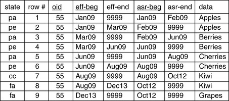 |
| Figure 15.1 A Bi-Temporal Table. |
Another three of those rows are no longer asserted. Their assertion periods are past. They represent claims that we once made, claims that the statements which those rows made about the objects which they represented were true statements. But now we no longer make those claims. They exist in the assertion time past. We designate these rows with “pa” (past asserted) in the state column of the table.
Two of those rows are not yet asserted. They are deferred assertions. We are not yet willing to claim that the statements made by those rows are true statements. We designate these rows with “fa” (future asserted) in the state column of the table.
There is one current row representing the object whose identifier is 55. This row is currently asserted and, within current assertion time, became effective in August 2009 and will remain in effect until further notice. Note, however, that it will remain asserted only until October 2012. At that time, if nothing in the data changes, the database will cease to say that the data for object 55 is Kiwi from August 2009 until further notice. Instead, it will say that data for object 55 is Kiwi from August 2009 to December 2013, and that from December 2013 until further notice, it will be Grapes. We designate this earlier, but current, row with “cc” (currently asserted current version) in the state metadata column of the table.
The SQL to retrieve the one current row for object 55 is:
SELECT data
FROM mytable
WHERE oid = 55
AND eff_beg_dt <= Now() AND eff_end_dt > Now()
AND asr_beg_dt <= Now() AND asr_end_dt > Now()
Most optimizers will use the index tree to locate the row id (rid) of the qualifying row or rows using, first of all, the columns that have direct matching predicates, such as EQUALS or IN, columns which are sometimes called match columns. These optimizers will also use the index tree for a column with a range predicate, such as BETWEEN or LESS THAN OR EQUAL TO (<=), provided that it is the first column in the index or the first column following the direct match columns.
Together, the direct match predicates and the first range predicate determine a starting position for a search of the index, that position being the first value found within the range specified on the first range predicate. And because of the match columns to the left of that first range column in the index, that first range predicate will direct us to the branch of the index tree where all the leaf node pointers point to rows in the target table which satisfy those match predicates as well that first range predicate. The most important thing to note here is that we get to this starting point in the search of the index without doing a scan. Our strategy is to get to the desired result using an index with little or no scanning.
Once we reach that starting point, all of the entries matching both the direct match predicates and also that first range predicate will be scanned. For all rows qualified by that scan, each of them will be scanned by the remaining predicates in the index. The index entries get narrowed down to a small set of pointers to all the rows in the table which match those search criteria whose columns appear on that index.
After the index scan is exhausted, it may still be necessary to scan the table itself. Although our goal is to have no scans at all, it isn't always possible to completely avoid them. Frequency of reads and updates, and other conditions, also need to be considered.
This is why the sequence of columns in an index is so important. Most important of all is to choose the correct range predicate column to place immediately after the common match predicate columns. To put the same point in other words: most important of all is to get positioned into the index for the desired row without resorting to scanning.
Suppose that the sequence of columns in the index is {oid, eff_beg_dt, asr_beg_dt}. In this case, using Figure 15.1, the optimizer will match on the 55, and then apply the less than or equal to predicate to the second indexed column, eff_beg_dt. If the current date is September 2011, there are eight rows where eff_beg_dt is less than or equal to the current date. So those eight rows will be scanned, and after that the other criteria will be applied while being scanned. Is this the best sequence of columns for this index, given that most queries will be looking for the one current row for an object, lost in a forest of non-current assertions and/or non-current versions for that same object?
In this proposed sequence of columns, the effective begin date immediately follows the match columns, and the next column is the assertion begin date. So after matching, and then filtering on effective begin date, the index will be scanned for the remaining criteria including assertion begin date. And the same eight rows will be qualified by that scan. Finally, the DBMS will use the row ids (rids) of the qualifying rows, and read the table itself. If the table is physically clustered on exactly this sequence of columns, we might get all eight rows in one I/O. On the other hand, in the worst case, it would require eight I/Os just to find the one current row. Since physical I/Os are one of the main causes of performance problems, reducing them is one of our main opportunities for optimization. And this particular sequence of index columns doesn't seem to do a good job in reducing I/O, either in the index or in the table itself.
Since there are probably more rows for object 55's past than for its future, we might consider reversing the sort order on the effective begin date index column, and make it descending instead of ascending. But even with a descending sort order, there are still the same eight rows that qualify and need further filtering. In fact, most rows in a temporal database usually have an effective begin date less than Now(). So effective begin date does not appear to be a good column to place immediately after the last match column in the index.
Another approach is to put all four temporal columns in the index. This might improve things, but it also has serious flaws. One problem is that some optimizers might ignore columns if the earlier columns do not match with EQUALS predicates (e.g. List Prefetch in earlier versions of DB2). And even if these four columns are used by the optimizer, an index scan may still be needed. Index performance for asserted version tables is most strongly affected by the one temporal column in the index that follows immediately after the match columns.
As we have now seen, effective begin date is not a good choice for that column position. Neither is assertion begin date, and for much the same reasons, as almost all rows have an assertion begin date earlier than the assertion begin date on the most frequently retrieved row, the current row for the object.
There are two remaining candidates for the column position that immediately follows the match columns: effective end date and assertion end date. In the table in Figure 15.1, there are the same number of rows with an assertion end date greater than Now() as there are rows with an effective end date greater than Now(). The ratio is determined by the number of updates to open-ended versions (ones with 12/31/9999 effective end dates) compared to the number of versions created with known effective end dates.
For example, a policy might have a known effective end date when it is created, whereas a client would normally not have one. So for a policy table, there would be fewer rows with an effective end date greater than Now(), because there would be fewer rows with a 12/31/9999 effective end date to withdraw into past assertion time. For a client table, it would be a toss-up. Since one withdrawn row is created for every temporal update, the number of rows for that object with an assertion end date greater than Now(), and the number of rows with an effective end date greater than Now() would tend to be roughly equal.
There is also an update performance issue with including the assertion end date anywhere in the index. Every time an episode is updated, a currently asserted row is withdrawn; and so its assertion end date is changed. This would require an update to the index, if the assertion end date is in that index; and it would happen every time a temporal update or a temporal delete is processed. By leaving the assertion end date out of the index, these frequent updates will not affect the index.
By a process of elimination, we have come to {oid, eff_end_dt} as the sequence of columns that will best optimize the performance of queries looking for the currently asserted current versions of objects. In this case, the optimizer will match on the 55, and then apply the GREATER THAN predicate to the second indexed column, eff_end_dt such as “eff_end_dt > Now()”. But for tables whose updates usually result in a version with a 12/31/9999 effective end date, the effective end date will not separate the currently asserted current version from the withdrawn versions for the same object. The best way to do that is to add the assertion end date as the last column in the index, giving us {oid, eff_end_dt, asr_end_dt}. Even though it will require an index scan to filter the assertions, doing so will often reduce the number of I/Os to the main table.
As we noted earlier, however, the assertion end date is updated every time a temporal update is carried out. It is updated as the then-current row is withdrawn into past assertion time, making room for the row or rows that replace it, or else replace and supercede it. So these physical updates will require a physical update to the corresponding index entry as well.
The decision of whether or not to include the assertion end date in an index designed to optimize access to the currently asserted current versions of objects, therefore, requires careful analysis of the specific situation. For policies and similar kinds of entities, where the effective end dates are usually known in advance, most withdrawn assertions will have an effective end date less than that of the currently asserted current version for the policy. This means that there is less need for the assertion end date in the index. But for clients and similar kinds of entities, where the effective end dates are usually not known in advance, many withdrawn assertions will contain an effective end date equal to that of the currently asserted current version, specifically the 12/31/9999 effective end date. This means that there is greater need for the assertion end date in the index, to push all those past assertions aside and allow us to get to the currently asserted current version more directly.
Generalizing from this specific case, our conclusion is that the sequence of columns for an asserted version table should begin with the match predicates for that table, starting with the most frequently used ones. After that, the effective end date should be the next column in the index. For tables in which most rows are created with a known (non-12/31/9999) effective end date, nothing else is needed in the index. But for tables in which most rows are created with a 12/31/9999, “until further notice”, effective end date, we recommend that the assertion end date be added to the index, right after the effective end date.
Currency Flags
Given the sensitivity of index use to range predicates, and the fact that currently asserted current versions will be the most frequently accessed (and frequently updated) rows in an asserted version table, it is tempting to consider the use of flags rather than dates to indicate currency. Flags can be used as match predicates, performing much better than dates used as range predicates.
Some implementations of historical data do use a flag to mark current rows. But this doesn't work for versions. For one thing, a current version can cease to be current with the passage of time. For another thing, if future versions are supported, they can become current with the passage of time. And it is impossible to guarantee that whenever a current version ceases to be current, the flag marking it as current will be changed on the exact clock tick when it stopped being current. Similarly, it is impossible to guarantee that whenever a future version becomes current, the flag marking it as non-current will be changed on the exact clock tick when it first becomes current.
For these reasons, currency flags are unreliable for versioned data. We cannot count on them to always tell us exactly which rows are current right now, and which rows are not. This may be acceptable for some business data requirements, but our implementation of Asserted Versioning is an enterprise solution, and must also work for databases where a request for current data will return current data no matter how recently it became current.
A currency flag doesn't work for assertions, either. Since asserted version tables support deferred transactions and deferred assertions, the same passage of time can move a currently asserted row into the past, and can also move a deferred assertion into current assertion time. And again, it is nearly impossible to maintain these flags on the exact clock tick when the change occurs. So there will be times when Now() does fall between begin and end dates, while currency flags indicate that it does not.
But as we will now explain, match predicate flags can be used in place of or in addition to range predicate dates in an index. A key insight is this: a currency flag must never classify a current row as non-current. But if that flag happens to classify a small number of non-current rows as current, that's not a problem. The objective for the index is to get us close for the most common access. The rest of the predicates in the query, or in the maintenance transaction, will get us all the way there, all the way to exactly the rows we want.
Using a Currency Flag to Optimize Queries
While many queries will look for versions that are no longer effective, or perhaps not yet effective, the vast majority of queries will look for versions that are currently asserted, versions that represent our best current knowledge of how things used to be, are, or may be at some point in the future. So it seems that there is greater potential improvement in query performance if we focus on assertion time.
We will call our current assertion time flag the circa flag (circa-asr-flag). It distinguishes between rows which are definitely known to be in the assertion time past from all other rows. All asserted version rows are created with an assertion begin date of Now() or an assertion begin date in the future. They are all created as either current assertions or deferred assertions. When they are created, their circa flag is set to ‘Y’, indicating that we cannot rule out the possibility that they are current assertions.
One way that a row can find itself in the assertion time past is for the AVF to withdraw that row in the process of completing a temporal update or a temporal delete transaction. When it does this, the AVF will also set that row's circa flag to ‘N’. At that point, both the flag and the row's assertion end date say the same thing. Both say that the row is definitely not a currently asserted row. (Both also say that the row is definitely not a deferred assertion, either; but the purpose of the flag is to narrow down the search for current assertions.)
The second way that a row can become part of past assertion time is by the simple passage of time. Whenever a temporal update transaction takes place, the assertion time specified on the transaction is used for both the assertion end date of the row being updated, and also for the assertion begin date of the row which updates it. Usually that assertion time is Now(), and so usually the result of the transaction is to immediately withdraw the row being updated into past assertion time and to immediately assert the row which supercedes it.
But when that temporal update is a deferred transaction, something different happens. Suppose that it is April 2013 right now, and a temporal update transaction is processed which has a future assertion date of July 2013. Just as with a non-deferred update, both the assertion end date of the version being updated, and also the assertion begin date of the version updating it, are given the assertion date specified on the transaction.
After this transaction, the original row has an assertion end date three months in the future. For those three months, it remains currently asserted. But after those three months have passed, i.e. once we are into the month of July 2013, that row will exist in the assertion time past. But it was not withdrawn; that is, it did not become assertion time past because of an explicit action on the part of the AVF. Instead, it has “fallen” into the past. We will say that it fell out of currency.
Because the row was not withdrawn by the AVF, its circa flag remains ‘Y’ even though its assertion end date has become earlier than Now(). And as long as its circa flag remains ‘Y’, this flag, by itself, will not exclude the row during an index search. However, as we will see, additional components come into play, components which will exclude that row.
Since the AVF itself cannot update circa flags on rows as they fall into the past, we will need to periodically run a separate process to find and update those flags. This can be done with the following SQL statement:
UPDATE mytable
SET circa_asr_flag = ‘N’
WHERE circa_asr_flag = ‘Y’
AND asr_end_dt < Now()
This update does not need to be run every second or every minute or every hour. It can be run as needed, during off hours such as nights or weekends, when system resources are more available.
How would we use this flag in an index? This flag could be used as the first column after the other direct matching columns in the index, for example: {oid, circa_asr_flag, eff_end_dt}. If the assertion end date were used instead of the circa flag, then the effective end date would require an index scan, prior to reaching the desired index entries. But by replacing the assertion end date with a match predicate, the effective end date becomes the first range predicate following the match predicates, and consequently can be processed without doing a scan.
Let's assume that it is now September 2011, and that the table we are querying is as shown in Figure 15.2. The circa flag has been added to the table shown in Figure 15.1, columns have been rearranged, and the rows from the original table have been resequenced on the index columns. Those columns are shown with their column headings shaded.
 |
| Figure 15.2 A Bi-Temporal Table with a Circa Flag. |
Note that row 7 has a non-12/31/9999 assertion end date. Its assertion end date is still in the future because the AVF processed a deferred temporal update against that row. That deferred temporal update created the deferred assertion which is row 8. In a year and a month, on October 2012, two rows will change their assertion time status, and will do so “quietly”, simply because of the passage of time. Row 7 will fall into the assertion time past and, at the same moment, row 8 will fall into the assertion time present.
Row 7 will cease to be currently asserted on that date. However, its circa flag will remain unchanged. As far as the flag can tell us, it remains a possibly current row. Also, row 8 will become currently asserted on that date. It was a possibly current row all along, and now it has become an actually current one. But its circa flag remains unchanged. That flag does not attempt to distinguish possibly current rows from actually current ones.
At some point, the SQL statement shown earlier will run. It will change the circa flag on row 7 to ‘N’, indicating that row 7 is definitely not a currently asserted row, and can never become one.
The following query will correctly filter and select the currently asserted current version of object 55 regardless of when the query is executed, and regardless of when the flag reset process is run. This is a query against the table shown in Figure 15.2 and let's assume that it is now September 2011.
SELECT data
FROM mytable
WHERE oid = 55
AND circa_asr_flag = ‘Y’
AND eff_beg_dt <= Now() AND eff_end_dt > Now()
AND asr_beg_dt <= Now() AND asr_end_dt > Now()
Processing this query, and using the index, the optimizer will:
(i) Match exactly on the predicate {oid = 55}
(ii) Match exactly on the predicate {circa_asr_flag= ‘Y’}; and
(iii) Then, using its first range predicate, {eff_end_dt > Now()}, it will position and start the index scan on the row with the first effective end date later than now, that row being row 8.
We have reached the first range predicate value, and have done so using only the index tree. At this point, an index scan begins; but we have already eliminated a large number of rows from the query's result set without doing any scanning at all.
When there are no more future effective versions found in the index scan, we will have assembled a list of index pointers to all rows which the index scan did not disqualify. But in this example, there is one more row with a future effective begin date, that being row 7. So, from its scan starting point, the index will scan rows 8, 7 and 9 and apply the other criteria. If some of the other columns are in the index, it will probably apply those filters via the index. If no other columns are in the index, it will go to the target table itself and apply the criteria that are not included in the index. Doing so, it will return a result set containing only row 7. Row 7's assertion end date has not yet been reached, so it is still currently asserted. And the assertion begin dates for rows 8 and 9 have not yet been reached, so they are not yet currently asserted.
In many cases, there will be no deferred assertions or future versions, and so the first row matched on the three indexed columns will be the only qualifying row. Whenever that is the case, we won't need the other temporal columns in the index. So restricting the index to just these three columns will keep the index smaller, enabling us to keep more of it in memory. This will improve performance for queries that retrieve the current row of objects that have no deferred assertions or future versions, but will be slightly slower when retrieving the current rows of objects that have either or both.
To understand how this index produces correct results whether it is run before or after the circa flag update process changes any flag values, let's assume that it is now November 2012, and the flag update process has not yet adjusted any flag values. In September, row 7 was the current row, and our use of the index correctly led us to that row. Now it is October, and the current row is row 9. Without any changes having been made to flag values, how does the index correctly lead us to this different result?
Prior to this tick of the clock, the table contained a current assertion with an October 2012 end date, and a deferred assertion with an October 2012 begin date. Because flag values haven't changed, our first three predicates will qualify the same three rows, rows 7, 8 and 9. But now row 7 will be filtered out because right now, November 2012 is past the assertion end date of October 2012. Row 9 will be filtered out because the effective begin date of December 2013 has not yet been reached. But row 8 meets all of the criteria and is therefore returned in the result set.
If the update of the circa flag is run on January 2013, let's say, it will change row 7's flag from ‘Y’ to ‘N’ because the assertion end date on that row is, when the process is run, in the past. Now, if our same query is run again, there will only be two rows to scan, two currently asserted rows. The SQL will correctly filter those two rows by their effective time periods, returning only the one row which is, at that time, also currently in effect.
Recall that the purpose of the circa flag is to optimize access to the most frequently requested data, that being current assertions about what things are currently like, i.e. currently asserted and currently effective rows. We note again that rows which make current assertions about what things are currently like are precisely the rows we find in non-temporal tables. Rather than being some exotic kind of bi-temporal construct, they are actually the “plain vanilla” data that is the only data found in most of the tables in a conventional database. For queries to such data, asserted version tables containing a circa flag, and having the index just described, will nearly match the performance of non-temporal tables.
Other Uses of the Circa Flag
While we have said that the purpose of this flag is to improve the performance of queries for currently asserted and currently effective data, it will also help the performance of queries for currently asserted but not currently effective versions by filtering out most withdrawn assertions and also versions no longer in effect as of the desired period of time. Another way to use the circa flag is to make it the first column in this index or in another index, and use it to create a separate partition for those past assertions whose circa flag also designates them as past. As we have said, this may not be all past assertions; but it will be most of them.
This will keep the index entries for current and deferred assertions together, and also separate from the index entries for assertions definitely known to be past assertions, resulting in a better buffer hit ratio. In fact, the index could be used as both a clustering and a partitioning index, in which case it would also keep more of the current rows in the target table in memory. To the circa flag eliminating definitely past assertions, and the oid column specifying the objects of interest, we also recommend adding the effective end date which will filter out past versions. The recommended clustering and partitioning index, then, is: {circa_asr_flag, oid, eff_end_dt}.
The circa flag can also be added to other search and foreign key indexes to help improve performance for current data. For example, a specialized index could be created to optimize searches for current Social Security Number data (currently asserted current versions of that data). The index would be: {SSN, circa_asr_flag, eff_end_dt}.
In this example, we have placed the circa flag after the SSN column so that index entries for all asserted version rows for the same SSN are grouped together. This means that the index will provide a slightly lower level of performance for queries looking for current SSN data than a {circa_asr_flag, oid, eff_end_dt} index, assuming we know the oid in addition to the SSN. But unlike that circa-first index, this index is also helpful for queries looking for as-was asserted data, that data being the mistakes we have made in our SSN data.
If we are looking for past assertions, it may also improve performance to code the circa flag using an IN clause. Some optimizers will manage short IN clause lists in an index look-aside buffer, effectively utilizing the predicate as though it were a match predicate rather than a range predicate.
In the following example, we follow standard conventions in showing program variables (e.g. those in a COBOL program's WORKING STORAGE section) as variable names preceded by the colon character. Also following COBOL conventions, we use hyphens in those variables. This convention was used, rather than generic Java or other dynamically prepared SQL with “?” parameter markers, to give an idea of the variables' contents.
SELECT data
FROM mytable
WHERE SSN = :my-ssn
AND eff_beg_dt <= :my-as-of-dt
AND eff_end_dt > :my-as-of-dt
AND asr_beg_dt <= :my-as-of-dt
AND assertion end date > :my-as-of-dt
AND circa_asr_flag IN (‘Y’, ‘N’)
In processing this query, a DB2 optimizer will first match on SSN. After that, still using the index tree rather than a scan, it will look aside for the effective end date under the ‘Y’ value for the circa flag, and then repeat the process for the ‘N’ value. This uses a matchcols of three; whereas without the IN clause, an index scan would begin right after the SSN match. However, we only recommend this for SQL where :my_as_of_dt is not guaranteed to be Now(). When that as-of date is Now(), using the EQUALS predicate ({circa_asr_flag = ‘Y’}) will perform much better since the ‘N’s do not need to be analyzed.
Query-enhancing indexes like these are not always needed. For the most part, as we said earlier, these indexes are specifically designed to improve the performance of queries that are looking for the currently asserted current versions of the objects they are interested in, and in systems that require extremely high read performance.
Indexes to Optimize Temporal Referential Integrity
Temporal referential integrity (TRI) is enforced in two directions. On the insert or temporal expansion of a child managed object, or on a change in the parent object designated by its temporal foreign key, we must insure that the parent object is present in every clock tick in which the child object is about to be present. On the deletion or temporal contraction of a parent managed object, we must RESTRICT, CASCADE or SET NULL that transformation so that it does not leave any “temporal orphans” after the transaction is complete.
In this section, we will discuss the performance considerations involved in creating indexes that support TRI checks on both parent and child managed objects.
Asserted Versioning's Non-Unique Primary Keys
First, and most obviously, each parent table needs an index whose initial column will be that table's object identifier (oid). The object identifier is also the initial column of the primary key (PK) of all asserted version tables. It is followed by two other primary key components, the effective begin date and the assertion begin date.
We need to remember that these physical PKs do not explicitly define the logical primary keys used by the AVF because the AVF uses date ranges and not specific dates or pairs of dates. Because of this, a unique index on the primary key of an asserted version table does not guarantee temporal entity integrity. These primary keys guarantee physical uniqueness; they guarantee that no two rows will have identical primary key values. But they do not guarantee semantic uniqueness, because they do not prevent multiple rows with the same object identifier from specifying [overlapping] or otherwise [intersecting] time periods.
The PK of an asserted version table can be any column or combination of columns that physically distinguish each row from all the other rows in the table. For example, the PK could be the object identifier plus a sequence number. It could be a single surrogate identity key column. It could be a business key plus the row create date. We have this freedom of choice because asserted version tables more clearly distinguish between semantically unique identifiers and physically unique identifiers than do conventional tables.
But this very freedom of choice poses a serious risk to any business deciding to implement its own Asserted Versioning framework. It is the risk of implementing Asserted Versioning's concepts one project at a time, one database at a time, one set of queries and maintenance transactions at a time. It is the risk of proliferating point solutions, each of which may work correctly, but which together pose serious difficulties for queries which range across two or more of those databases. It is the risk of failing to create an enterprise implementation of bi-temporal data management.
The semantically unique identifier for any asserted version table is the combination of the table's object identifier and its two time periods. And to emphasize this very important point once again: two pairs of dates are indeed used to represent two time periods, but they are not equivalent to two time periods. What turns those pairs of dates into time periods is the Asserted Versioning code which guarantees that they are treated as the begin and end delimiters for time periods.
Given that there should be one enterprise-wide approach for Asserted Versioning primary keys, what should it be? First of all, an enterprise approach requires that the PK of an asserted version table must not contain any business data. The reason is that if business data were used, we could not guarantee that the same number of columns would be used as the PK from one asserted version table to the next, or that column datatypes would even be the same. These differences would completely eliminate the interoperability benefits which are one of the objectives of an enterprise implementation. But beyond that restriction, the choice of an enterprise standard for Asserted Versioning primary keys, in a proprietary implementation of Asserted Versioning concepts, is up to the organization implementing it.
We have now shown how the choice of columns beyond the object identifier—the choice of the effective end date and the assertion end date, and optionally a circa flag—is used to minimize scan costs in both indexes and the tables they index. We next consider, more specifically, indexes whose main purpose is to support the checks which enforce temporal referential integrity.
Indexes on TRI Parents
As we have explained, a temporal foreign key (TFK) never contains a full PK value. So it never points to a specific parent row. This is the principal way in which it is different from a conventional foreign key (FK), and the reason that current DBMSs cannot enforce temporal referential integrity.
A complete Asserted Versioning temporal foreign key is a combination of a column of data and a function. That column of data contains the object identifier of the object on which the child object is existence-dependent. That function interprets pairs of dates on the child row being created (by either an insert or an update transaction) as time periods, and pairs of dates on the parent episode as time periods. With that information, the AVF enforces TRI, insuring that any transformation of the database will leave it in a state in which the full extent of a child version's time periods are included within its parent episode's time periods. It also enforces temporal entity integrity (TEI), insuring that no two rows representing the same object ever share a pair of assertion time and effective time clock ticks.
The AVF needs an index on the parent table to boost the performance of its TRI enforcement code. We do not want to perform scans while trying to determine if a parent object identifier exists, and if the effective period of the dependent is included within a single episode of the parent. The most important part of this index on the parent table is that it starts with the object identifier.
The AVF uses the object identifier and three temporal dates. First, it uses the parent table's episode begin date, rather than its effective begin date, because all TRI time period comparisons are between a child version and a parent episode. So we will consider the index sequence as described earlier to reduce scans, but then add the episode begin date.
Instead of creating a separate index for TRI parent-side tables, we could try to minimize the number of indexes by re-using the primary key index to:
(i) Support uniqueness for a row, because some DBMS applications require a unique PK index for single-row identification.
(ii) Help the AVF perform well when an object is queried by its object identifier; and
(iii) Improve performance for the AVF during TRI enforcement.
So we recommend an index whose first column is the object identifier of the parent table. Our proposed index is now {oid, . . . . .}. Next, we need to determine if we expect current data reads to the table to outnumber non-current reads or updates.
If we expect current data reads to dominate, then the next column we might choose to use is the circa flag. If this flag is used as a higher-level node in the index, then TRI maintenance in the AVF can use the {circa_asr_flag = ‘Y’} predicate to ignore most of the rows in past assertion time. This could significantly help the performance of TRI maintenance. Using the circa flag, our proposed index is now {oid, circa_asr_flag. . . . .}. The assumption here is that the DBMS allows updates to a PK value with no physical foreign key dependents because the circa flag will be updated.
Just as in any physical data modeling effort, the DBA or Data Architect will need to analyze the tradeoffs of indexing for reads vs. indexing for updates. The decision might be to replace a single multi-use index with several indexes each supporting a different pattern of access. But in constructing an index to help the performance of TRI enforcement, the next column should be the effective end date, for the reasons described earlier in this chapter. Our proposed index is now {oid, circa_asr_flag, eff_end_dt, . . . . .}.
After that, the sequence of the columns doesn't matter much because the effective end date is used with a range predicate, so direct index matching stops there. However, other columns are needed for uniqueness, and the optimizer will still likely use any additional columns that are in the index and qualified as criteria, filtering on everything it got during the index scan rather than during the more expensive table scan.
If the circa flag is not included in the index, and the DBMS allows the update of a primary key (with no physical dependents), then the next column should be the assertion end date. Otherwise, the next column should be the assertion begin date. In either case, we now have a unique index, which can be used as the PK index, for queries and also for TRI enforcement. Finally, to help with TRI enforcement, we recommend adding the episode begin date. This is because the parent managed object in any TRI relationship is always an episode.
Depending on whether or not the circa flag is included, this unique index is either
{oid, circa_asr_flag, eff_end_dt, asr_beg_dt, epis_beg_dt}
or
{oid, eff_end_dt, asr_end_dt, epis_beg_dt}
Let's be sure we understand why both indexes are unique. The unique identifier of any object is the combination of its oid, assertion time period and effective time period. In the primary key of asserted version tables, those two time periods are represented by their respective begin dates. But because the AVF enforces temporal entity integrity, no two rows for the same object can share both an assertion clock tick and an effective clock tick. So in the case of these two indexes, while the assertion begin date represents the assertion time period, the effective end date represents the effective time period. Both indexes contain an object identifier and one delimiter date representing each of the two time periods, and so both indexes are unique.
Indexes on TRI Children
Some DBMSs automatically create indexes for foreign keys declared to the DBMS, but others do not. Regardless, since Asserted Versioning does not declare its temporal foreign keys using SQL's Data Definition Language (DDL), we must create our own indexes to improve the performance of TRI enforcement on TFKs.
Each table that contains a TFK should have an index on the TFK columns primarily to assist with delete rule enforcement, such as ON DELETE RESTRICT, CASCADE or SET NULL. These indexes can be multi-purpose as well, also being used to assist with general queries that use the oid value of the TFK. We should try to design these indexes to support both cases in order to minimize the system overhead otherwise required to maintain multiple indexes.
When a temporal delete rule is fired from the parent, it will look at every dependent table that uses the parent's oid. It will also use the four temporal dates to find rows that fall within the assertion and effective periods of the related parent.
The predicate to find dependents in any contained clock tick would look something like this:
WHERE parent_oid = :parent-oid
AND eff_beg_dt < :parent-eff-end-dt
AND eff_end_dt > :parent-eff-beg-dt
AND circa_asr_flag = ‘Y’ (if used)
AND asr_end_dt >= Now()
(might have deferred assertion criteria, too)
In this SQL, the columns designated as parent dates are the effective begin and end dates specified on the delete transaction.
In an index designed to enhance the performance of the search for TRI parent–child relationships, the first column should be the TFK. This is the oid value that relates a child to a parent.
Temporal referential integrity checks are never concerned with withdrawn assertions, so this is another index in which the circa flag will help performance. If we use this flag, it should be the next column in the index. However, if this is the column that will be used for clustering or partitioning, the circa flag should be listed first, before the oid.
For TRI enforcement, the AVF does not use a simple BETWEEN predicate because it needs to find dependents with any overlapping clock ticks. Instead, it uses an [intersects] predicate.
Two rules used during TRI delete enforcement are that the effective begin date on the episode must be less than the effective end date specified on the delete transaction, and that the effective end date on the episode must be greater than the effective begin date on the transaction.
Earlier, we pointed out that for current data queries, there are usually many more historical rows than current and future rows, and for that reason we made the next column the effective end date rather than the effective begin date. These same considerations hold true for indexes assisting with temporal delete transactions.
Therefore, our recommended index structure for TFK indexes, which can be used for both TRI enforcement by the AVF, and also for any queries looking for parent object and child object relationships, where the oid mentioned is the TFK value, is either {parent_oid, circa_asr_flag, eff_end_dt. . . . .} or {parent_oid, eff_end_dt, asr_end_dt. . . . .}.
Other temporal columns could be added, depending on application-specific uses for the index.
Other Techniques for Performance Tuning Bi-Temporal Tables
In an Asserted Versioning database, most of the activity is row insertion. No rows are physically deleted; and except for the update of the assertion end date when an assertion is withdrawn, or the update of the assertion begin date when far future deferred assertions are moved into the near future, there are no physical updates either. On the other hand, there are plenty of reads, usually to current data. We need to consider these types of access, and their relative frequencies, when we decide which optimization techniques to use.
Avoiding MAX(dt) Predicates
Even if Asserted Versioning did not support logical gap versioning, we would keep both effective end dates and assertion end dates in the Asserted Versioning bi-temporal schema. The reason is that, without them, most accesses to these tables would require finding the MAX(dt) of the designated object in assertion time, or in effective time within a specified period of assertion time. The performance problem with a MAX(dt) is that it needs to be evaluated for each row that is looked at, causing performance degradation exponential to the number of rows reviewed.
Experience with the AVF and our Asserted Versioning databases has shown us that eliminating MAX(dt) subqueries and having effective and assertion end dates on asserted version tables, dramatically improves performance.
NULL vs. 12/31/9999
Some readers might wonder why we do not use nulls to stand in for unknown future dates, whether effective end dates or assertion end dates. From a logical point of view, NULL, which is a marker representing the absence of information, is what we should use in these date columns whenever we do not know what those future dates will be.
But experience with the AVF and with Asserted Versioning databases has shown that using real dates rather than nulls helps the optimizer to consistently choose better, more efficient access paths, and matches on index keys more directly.
Without using NULL, the predicate to find versions that are still in effect is:
eff_end_dt > Now()
Using NULL, the semantically identical predicate is:
(eff_end_dt > Now() OR eff_end_dt IS NULL)
The OR in the second example causes the optimizer to try one path and then another. It might use index look-aside, or it might scan. Either of these is less efficient than a single GREATER THAN comparison.
Another considered approach is to coalesce NULL and the latest date recognizable by the DBMS, giving us the following predicate:
COALESCE(eff_end_dt, ‘12/31/9999’) > Now()
But functions normally cannot be resolved in standard indexes, and so the COALESCE function will normally cause a scan. Worse yet, some DBMSs will not resolve functions until all data is read and joined. So frequently, a lot of extra data will be assembled into a preliminary result set before this COALESCE function is ever applied.
The last of our three options is a simple range predicate (such as GREATER THAN) without an OR, and without a function. If the end date is unknown, and the value we use to represent that unknown condition is the highest date (or timestamp) which the DBMS can recognize, then this simple range predicate will return the same results as the other two predicates. And given that the highest date a DBMS can recognize is likely to be far into the future, it is unlikely that business applications will ever need to use that date to represent that far-off time. In SQL Server, for example, that highest date is 12/31/9999. So as long as our business applications do not need to designate that specific New Year's Eve nearly 8000 years from now, we are free to use it to represent the fact that a value is unknown. Using it, we can use the simple range predicate shown earlier in this section, and reap the benefits of the excellent performance of that kind of predicate.
Partitioning
Another technique that can help with performance and database maintenance, such as backups, recoveries and reorganizations, is partitioning. There are several basic approaches to partitioning.
One is to partition by a date, or something similar, so that the more current and active data is grouped together, and is more likely to be found in cache. This is a common partitioning strategy for on-line transaction processing systems.
Another is to partition by some known field that could keep commonly accessed smaller groups of data together, such as a low cardinality foreign key. The benefit of this approach is that it directs a search to a small well-focused collection of data located on the same or on adjacent I/O pages. This strategy improves performance by taking advantage of sequential prefetch algorithms.
A third approach is to partition by some random field to take advantage of the parallelism in data access that some DBMSs support. For these DBMSs, the partitions define parallel access paths. This is a good strategy for applications such as reporting and business intelligence (BI) where typically large scans could benefit from the parallel processing made possible by the partitioning.
Some DBMSs require that the partitioning index also be the clustering index. This limits options because it forces a trade-off between optimizing for sequential prefetch and optimizing for parallel access. Fortunately, DBMS vendors are starting to separate the implementation of these two requirements.
Another limitation of some DBMSs, but one that is gradually being addressed by their vendors, is that whenever a row is moved between partitions, those entire partitions are both locked. This forces application developers to design their processes so that they never update a partitioning key value on a row during prime time, because doing so locks the source and destination partitions until the move is complete. As we noted, more recent releases of DBMSs reduce the locking required to move a row from one partition to another.
A good partitioning strategy for an Asserted Versioning database is to partition by one of the temporal columns, such as the assertion end date, in order to keep the most frequently accessed data in cache. As we have pointed out, that will normally be currently asserted current versions of the objects of interest to the query.
For an optimizer to know which partition(s) to access, it needs to know the high order of the key. For direct access to the other search criteria, it needs direct access to the higher nodes in the key, higher than the search key. Therefore, while one of the temporal dates is good for partitioning, it reduces the effectiveness of other search criteria. To avoid this problem, we might want to define two indexes, one for partitioning, and another for searching.
The better solution for defining partitions that optimize access to currently asserted versions is to use the circa flag as the first column in the partitioning index. The best predicate would be {circa_asr_flag = ‘Y’} for current assertions. For DBMSs which support index-look-aside processing for IN predicates, the best predicate might be {circa_asr_flag IN (‘Y’, ‘N’)} when it is uncertain if the version is currently asserted. With this predicate, the index can support searches for past assertions as well as searches for current ones. Otherwise, it will require a separate index to support searches for past assertions.
Clustering
Clustering and partitioning often go together, depending on the reason for partitioning and the way in which specific DBMSs support it. Whether or not partitioning is used, choosing the best clustering sequence can dramatically reduce I/O and improve performance.
The general concept behind clustering is that as the database is modified, the DBMS will attempt to keep the data on physical pages in the same order as that specified in the clustering index. But each DBMS does this a little differently. One DBMS will cluster each time an insert or update is processed. Another will make a valiant attempt to do that. A third will only cluster when the table is reorganized. But regardless of the approach, the result is to reduce physical I/O by locating data that is frequently accessed together as physically close together as possible.
Early DBMSs only allowed one clustering index, but newer releases often support multiple clustering sequences, sometimes called indexed views or multi-dimensional clustering.
It is important to determine the most frequently used access paths to the data. Often the most frequently used access paths are ones based on one or more foreign keys. For asserted version tables, currently asserted current versions are usually the most frequently queried data.
Sometimes, the right combination of foreign keys can provide good clustering for more than one access path. For example, suppose that a policy table has two low cardinality TFKs, product type and market segment, and that each TFK value has thousands of related policies. 3 We might then create this clustering index:
{circa_asr_flag, product_type_oid, market_segment_oid, eff_end_dt, policy_oid}
3Low cardinality means that there are fewer distinct values for the field in the table which results in more rows having a single value.
The circa flag would cluster most of the currently asserted rows together, keeping them physically co-located under the lower cardinality columns. Clustering would continue based on effective date, and then by the higher cardinality object identifier of the table. This will provide access via the product type oid, and will tend to cluster the data for current access for three other potential search indexes:
(i) {product_type_oid, circa_asr_flag, eff_end_dt};
(ii) {market_segment_oid, circa_asr_flag, eff_end_dt}; or
(iii) {policy_oid, circa_asr_flag, eff_end_dt}.
Materialized Query Tables
Materialized Query Tables (MQTs), sometimes called Indexed Views, are extremely helpful in optimizing the performance of Asserted Versioning databases. They are especially helpful when querying currently asserted current versions.
Some optimizers will automatically determine if an MQT can be used, even if we do not explicitly specify one in the SQL FROM clause. Some DBMSs will let us specifically reference an MQT. Certain implementations of MQTs do not allow volatile variables and system registers, such as Now() or CURRENT TIMESTAMP in the definition, because the MQTs would be in a constant rebuild state. For example, we could not code the following in the definition of the MQT:
asr_end_dt > Now()
However, we could code a literal such as:
asr_end_dt > ‘01/01/2010’
This would work, but obviously the MQT would have to be recreated each time the date changed. Another option is to create a single row table with today's date in it, and join to that table. For example, consider a Today table with a column called today's date. An MQT table would be joined to this table using a predicate like {asr_end_dt > Today.todays_dt}. Then, we could periodically increment the value of todays_dt to rebuild the MQT.
However, this is another place where we recommend the circa flag. If we have it, we can just use the {circa_asr_flag = ‘Y’} predicate in the MQT definition. This will keep the overhead low, will keep maintenance to a minimum, and will segregate past assertion time data, thereby getting better cache/buffer utilization.
We can also create something similar to the circa flag for the effective end date. This would be used to include currently effective versions in an MQT. However, for the same reasons we cannot use Now() in an assertion time predicate, we cannot use {eff_end_dt > Now()} in MQT definitions because of the volatile system variable Now(). So instead, we can use an effective time flag, and code a {circa_eff_flag = ‘Y’} predicate in the MQT definition.
MQTs could also be helpful when joining multiple asserted version tables together.
With most MQT tables, we have a choice of refreshing them either periodically or immediately. Our choice depends on what the DBMS permits, and the requirements of specific applications and specific MQTs.
Standard Tuning Techniques
In addition to tuning techniques specific to Asserted Versioning databases, there are general tuning techniques that are just as applicable to temporal tables as to conventional or non-temporal ones.
Use Cache Profligately. Per-unit memory costs, like per-unit costs for other hardware components, are falling. Multi-gigabyte memory is now commonplace on personal computers, and terabyte memories are now found on mainframe computers. Try to get as many and as much of your indexes in cached buffers as you can. Reducing physical I/O is essential to good performance.
Use Parameter Markers. If we cannot use static SQL for a frequently executed large data volume query, then the next best thing is to prepare the SQL with parameter markers. Many optimizers will perform a hashed compare of the SQL to the database dynamic prepared SQL cache, then a direct compare of the SQL being prepared, looking for a match. If it finds a match, it will avoid the expensive access path determination optimization process, and will instead use the previously determined access path rather than trying to re-optimize it.
The reason for the use of parameter markers rather than literals for local predicates is that with cache matching, the optimizer is much more likely to find a match. For example, a prepared statement of does not match causing the statement to be re-optimized. But a prepared SQL statement of will find a match whether the value of the parameter marker is 44, 55, or any other number, and in most cases will not need to be re-optimized.
SELECT * FROM mytable WHERE oid = 55
SELECT * FROM mytable WHERE oid = 44
SELECT * FROM mytable WHERE oid = ?
Use More Indexes. Index other common search columns such as business keys. Also, use composite key indexes when certain combinations of criteria are often used together.
Eliminate Sorts. Try to reduce DBMS sorting by having index keys match the ORDER BY or GROUP BY sequence after EQUALS predicates.
Explain/Show Plan. Know the estimated execution time of the SQL. Incorporate SQL tuning into the system development life cycle.
Monitor and Tune. Some monitoring tools will identify the SQL statements that use the most overall resources. But as well as the single execution overhead identified in the Explain (Show Plan), it is important to also consider the frequency of execution of the SQL statements. For example, a SQL statement that runs for 6 seconds but is called only 10 times per hour uses a lot fewer resources than another that runs only 60 milliseconds, but is called 10,000 times per hour—in this case, 1 minute vs. 10 minutes total time. The query it is most important to optimize is the 60 millisecond query.
Use Optimization Hints Cautiously. Most optimizers work well most of the time. However, once in a while, they just don't get it right. It's getting harder to force the optimizer into choosing a better access path, for example by using different logical expressions with the same truth conditions, or by fudging catalog statistics. However, most optimizers support some type of optimization hints. Use them sparingly, but when all else fails, and the optimizer is being stubborn, use them.
Use Isolation Levels. Specify the appropriate Isolation Level to minimize locks and lock waits. Isolation levels of Cursor Stability (CS) or Uncommitted Read (UR) can significantly improve the throughput compared to more restrictive levels such as Repeatable Read (RR). However, keep in mind that a temporal update usually expands into several physical inserts and updates to the objects. So make sure that less restrictive isolation levels are acceptable to the application.
Glossary References
Glossary entries whose definitions form strong inter-dependencies are grouped together in the following list. The same glossary entries may be grouped together in different ways at the end of different chapters, each grouping reflecting the semantic perspective of each chapter. There will usually be several other, and often many other, glossary entries that are not included in the list, and we recommend that the Glossary be consulted whenever an unfamiliar term is encountered.
12/31/9999
Asserted Versioning Framework (AVF)
assertion
assertion begin date
assertion end date
assertion time period
bi-temporal database
conventional database
non-temporal database
circa flag
clock tick
time period
deferred assertion
effective begin date
effective end date
effective time period
episode begin date
object
object identifier
oid
fall out of currency
withdraw
temporal column
temporal entity integrity (TEI)
temporal foreign key (TFK)
temporal referential integrity (TRI)
version
..................Content has been hidden....................
You can't read the all page of ebook, please click here login for view all page.