7.2 One-Sample t-Interval for the Mean
7.3 One-Sample t-Test for the Mean
7.4 Two-Sample t-Interval for the Difference Between Two Means
7.5 Two-Sample t-Test for the Difference Between Two Means
7.6 Matched Pairs (One-Sample t)
7.7 Errors in Hypothesis Testing: Type I, Type II, and Power
![]() The Central Limit Theorem (CLT) is a very powerful tool, as was evident in the previous chapter. Our penny activity demonstrated that as long as we have a large enough sample, the sampling distribution of
The Central Limit Theorem (CLT) is a very powerful tool, as was evident in the previous chapter. Our penny activity demonstrated that as long as we have a large enough sample, the sampling distribution of ![]() is approximately normal. This is true no matter what the population distribution looks like. To use a z-statistic, however, we have to know the population standard deviation, σ. In the real world, σ is usually unknown. Remember, we use statistical inference to make predictions about what we believe to be true about a population.
is approximately normal. This is true no matter what the population distribution looks like. To use a z-statistic, however, we have to know the population standard deviation, σ. In the real world, σ is usually unknown. Remember, we use statistical inference to make predictions about what we believe to be true about a population.
![]() When σ is unknown, we estimate σ with s. Recall that s is the sample standard deviation. When using s to estimate σ, the standard deviation of the sampling distribution for means is
When σ is unknown, we estimate σ with s. Recall that s is the sample standard deviation. When using s to estimate σ, the standard deviation of the sampling distribution for means is ![]() . When you use s to estimate σ, the standard deviation of the sampling distribution is called the standard error of the sample mean,
. When you use s to estimate σ, the standard deviation of the sampling distribution is called the standard error of the sample mean, ![]() .
.
![]() While working for Guinness Brewing in Dublin, Ireland, William S. Gosset discovered that when he used s to estimate σ, the shape of the sampling distribution changed depending on the sample size. This new distribution was not exactly normal. Gosset called this new distribution the t-distribution. It is sometimes referred to as the student’s t.
While working for Guinness Brewing in Dublin, Ireland, William S. Gosset discovered that when he used s to estimate σ, the shape of the sampling distribution changed depending on the sample size. This new distribution was not exactly normal. Gosset called this new distribution the t-distribution. It is sometimes referred to as the student’s t.
![]() The t-distribution, like the standard normal distribution, is single-peaked, symmetrical, and bell shaped. It’s important to notice, as mentioned earlier, that as the sample size (n) increases, the variability of the sampling distribution decreases. Thus, as the sample size increases, the t-distributions approach the standard normal model. When the sample size is small, there is more variability in the sampling distribution, and therefore there is more area (probability) under the density curve in the “tails” of the distribution. Since the area in the “tails” of the distribution is greater, the t-distributions are “flatter” than the standard normal curve. We refer to a t-distribution by its degrees of freedom. There are n−1 degrees of freedom. The “n−1” degrees of freedom are used since we are using s to estimate σ and s has n−1 degrees of freedom. Figure 7.1 shows two different t-distributions with 3 and 12 degrees of freedom, respectively, along with the standard normal curve. It’s important to note that when dealing with a normal distribution,
The t-distribution, like the standard normal distribution, is single-peaked, symmetrical, and bell shaped. It’s important to notice, as mentioned earlier, that as the sample size (n) increases, the variability of the sampling distribution decreases. Thus, as the sample size increases, the t-distributions approach the standard normal model. When the sample size is small, there is more variability in the sampling distribution, and therefore there is more area (probability) under the density curve in the “tails” of the distribution. Since the area in the “tails” of the distribution is greater, the t-distributions are “flatter” than the standard normal curve. We refer to a t-distribution by its degrees of freedom. There are n−1 degrees of freedom. The “n−1” degrees of freedom are used since we are using s to estimate σ and s has n−1 degrees of freedom. Figure 7.1 shows two different t-distributions with 3 and 12 degrees of freedom, respectively, along with the standard normal curve. It’s important to note that when dealing with a normal distribution,  Using s to estimate σ introduces another source of variability into the statistic.

![]() As mentioned earlier, we use statistical inference when we wish to estimate some parameter of the population. Often, we want to estimate the mean of a population. Since we know that sample statistics usually vary, we will construct a confidence interval. The confidence interval will give a range of values that would be reasonable values for the parameter of interest, based on the statistic obtained from the sample. In this section, we will focus on creating a confidence interval for the mean of a population.
As mentioned earlier, we use statistical inference when we wish to estimate some parameter of the population. Often, we want to estimate the mean of a population. Since we know that sample statistics usually vary, we will construct a confidence interval. The confidence interval will give a range of values that would be reasonable values for the parameter of interest, based on the statistic obtained from the sample. In this section, we will focus on creating a confidence interval for the mean of a population.
![]() When dealing with inference, we must always check certain assumptions for inference. This is imperative! These “assumptions” must be met for our inference to be reliable. We confirm or disconfirm these “assumptions” by checking the appropriate conditions. Throughout the remainder of this book, we will perform inference for different parameters of populations. We must always check that the assumptions are met before we draw conclusions about our population of interest. If the assumptions cannot be verified, our results may be inaccurate. For each type of inference, we will discuss the necessary assumptions and conditions.
When dealing with inference, we must always check certain assumptions for inference. This is imperative! These “assumptions” must be met for our inference to be reliable. We confirm or disconfirm these “assumptions” by checking the appropriate conditions. Throughout the remainder of this book, we will perform inference for different parameters of populations. We must always check that the assumptions are met before we draw conclusions about our population of interest. If the assumptions cannot be verified, our results may be inaccurate. For each type of inference, we will discuss the necessary assumptions and conditions.
![]() The assumptions and conditions for a one-sample t-interval or one-sample t-test are as follows:
The assumptions and conditions for a one-sample t-interval or one-sample t-test are as follows:
Assumptions 1. Individuals are independent | Conditions 1. SRS and <10% of population (10n<N) |
2. Normal population assumption | 2. One of the following:
|
![]() The t-procedures (t-interval and t-test) are robust, meaning that the results of our t-interval or t-test would not change very much even though the assumptions of the procedure are violated.
The t-procedures (t-interval and t-test) are robust, meaning that the results of our t-interval or t-test would not change very much even though the assumptions of the procedure are violated.
![]() Let’s discuss the assumptions and conditions. The first assumption is that the individuals or observations are independent. This should be true if our sample data is an SRS or if our data comes from a randomized experiment and if the sample size is less than 10% of the population size. The second assumption is that the population is normal. We may know or be given that the population is normal. If this is the case, we state this in our problem. If we do not know or if we are not told that the population is normal and the sample size is small, we must then look at a graph of the sample data. A histogram or a modified boxplot is probably best suited for looking at the sample data. If the sample size is less than 30, we must be cautious of outliers or skewness in the data. Since normal distributions drop off quickly, it is unlikely to take a sample from a normal population and have the sample contain outliers or skewness. Outliers and strong skewness in a sample can be an indication that the population from which the sample is drawn might be non-normal. If the sample is large, we know that no matter what the population distribution looks like, we are guaranteed that the sampling distribution will be approximately normal. If you are asked to work on a problem for which the assumptions cannot be verified, state that this is the case and that the results of the inference being performed may be inaccurate.
Let’s discuss the assumptions and conditions. The first assumption is that the individuals or observations are independent. This should be true if our sample data is an SRS or if our data comes from a randomized experiment and if the sample size is less than 10% of the population size. The second assumption is that the population is normal. We may know or be given that the population is normal. If this is the case, we state this in our problem. If we do not know or if we are not told that the population is normal and the sample size is small, we must then look at a graph of the sample data. A histogram or a modified boxplot is probably best suited for looking at the sample data. If the sample size is less than 30, we must be cautious of outliers or skewness in the data. Since normal distributions drop off quickly, it is unlikely to take a sample from a normal population and have the sample contain outliers or skewness. Outliers and strong skewness in a sample can be an indication that the population from which the sample is drawn might be non-normal. If the sample is large, we know that no matter what the population distribution looks like, we are guaranteed that the sampling distribution will be approximately normal. If you are asked to work on a problem for which the assumptions cannot be verified, state that this is the case and that the results of the inference being performed may be inaccurate.
![]() The following example involves finding a confidence interval. As you solve statistical inference problems in this and the following chapters, keep in mind the following three steps:
The following example involves finding a confidence interval. As you solve statistical inference problems in this and the following chapters, keep in mind the following three steps:
Identify the parameter of interest, choose the appropriate inference procedure, and verify that the assumptions and conditions for that procedure are met.
Carry out the inference procedure. Do the math! Be sure to apply the correct formula.
Interpret the results in the context of the problem.
![]() Example 1: Nolan wanted to estimate the average number of miles that a typical Indiana high-school male cross-country runner would run over a one-week period. The following is a random sample of the number of miles per week run by 20 male high-school cross-country runners in the state of Indiana. Find a 90% confidence interval for the average number of miles run per week for all male high-school cross-country runners in the state of Indiana.
Example 1: Nolan wanted to estimate the average number of miles that a typical Indiana high-school male cross-country runner would run over a one-week period. The following is a random sample of the number of miles per week run by 20 male high-school cross-country runners in the state of Indiana. Find a 90% confidence interval for the average number of miles run per week for all male high-school cross-country runners in the state of Indiana.
20, 30, 35, 40, 40, 45, 45, 45, 50, 50, 50, 50, 52, 54, 55, 60, 60, 60, 70, 75
Solution:
Step 1: Find a 90% confidence interval for μ the mean number of miles run per week by a male high-school cross-country runner in the state of Indiana. Since σ is unknown, we will use a one-sample t-interval for the mean. We must check the assumptions and conditions.
Assumptions and conditions that verify:
Individuals are independent. We are given that the sample is random, and we can safely assume that there are more than 200 male crosscountry runners in the state of Indiana (10n < N).
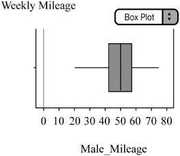
Normal population assumption. We are given a small sample, but a modified boxplot of the sample data appears to be symmetric with no outliers (Figure 7.2). We should be safe using t-procedures.
Step 2: Since the conditions are met, we will construct the confidence interval for the population mean, μ, using:
![]()
t* = 1.729 can be found by using the t-distribution table. Use 19 df and cross-reference with 90% confidence at the bottom of the table. Study the table. Notice how the t* values increase and approach z* as the degrees of freedom and the sample size increase. Remember that the t-distributions approach the normal distribution when the sample size gets large.
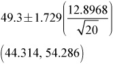
Step 3: Conclude in context! We are 90% confident that the true average number of miles that Indiana high-school male cross-country runners run in a given week is between 44.314 and 54.286 miles (“true average” refers to the average of all Indiana male cross-country runners).
![]() Notice that the sample mean,
Notice that the sample mean, ![]() , is the center of the confidence interval. The distance between the ends of the confidence interval and the center is called the margin of error. Thus,
, is the center of the confidence interval. The distance between the ends of the confidence interval and the center is called the margin of error. Thus, ![]() is the margin of error.
is the margin of error.
![]() I highly recommend using the three-step process when doing inference. Some textbooks write up the inference problems a little differently. As long as you have all the essentials of the inference procedure, it doesn’t make a huge difference how you organize it. I have found it best to find a system you can use so that you don’t leave out any of the essentials of inference, including the assumptions and conditions. Always show your work!
I highly recommend using the three-step process when doing inference. Some textbooks write up the inference problems a little differently. As long as you have all the essentials of the inference procedure, it doesn’t make a huge difference how you organize it. I have found it best to find a system you can use so that you don’t leave out any of the essentials of inference, including the assumptions and conditions. Always show your work!
![]() Refer to Example 1; it’s important to note several things. First of all, make sure you define any variables you use. State what procedure you are going to use and, of course, make sure you check the assumptions and conditions. If you refer to a histogram, modified boxplot, or any type of graph of the data, make sure to include the graph. Don’t assume that the reader (grader) will know what you are talking about. Always plot the data if you are given a small sample. If the sample is over 30 (some books say 40), then you do not have to plot the sample data. Remember that if the sample is “large enough,” then the sampling distribution should be approximately normal, no matter what the sample data looks like. If the population is given to be normal, you don’t have to worry about skewness or outliers either. If you are not given a normal population and the sample is less than 30, then you must plot the sample data to look for skewness and outliers.
Refer to Example 1; it’s important to note several things. First of all, make sure you define any variables you use. State what procedure you are going to use and, of course, make sure you check the assumptions and conditions. If you refer to a histogram, modified boxplot, or any type of graph of the data, make sure to include the graph. Don’t assume that the reader (grader) will know what you are talking about. Always plot the data if you are given a small sample. If the sample is over 30 (some books say 40), then you do not have to plot the sample data. Remember that if the sample is “large enough,” then the sampling distribution should be approximately normal, no matter what the sample data looks like. If the population is given to be normal, you don’t have to worry about skewness or outliers either. If you are not given a normal population and the sample is less than 30, then you must plot the sample data to look for skewness and outliers.
![]() Note that a graphing calculator could be used to find the confidence interval. It can also perform various tests of significance. The graphing calculator is a powerful tool, but it doesn’t take the place of applying formulas and showing our work.
Note that a graphing calculator could be used to find the confidence interval. It can also perform various tests of significance. The graphing calculator is a powerful tool, but it doesn’t take the place of applying formulas and showing our work.
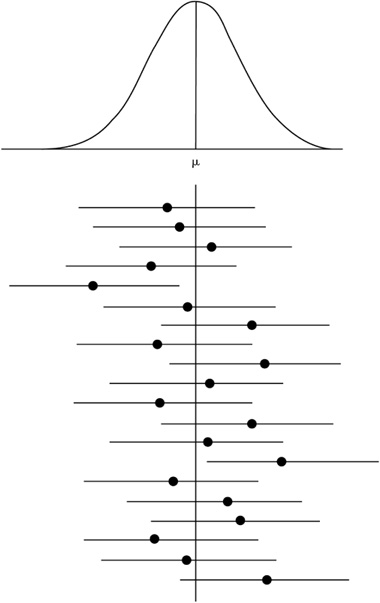
![]() It is highly likely that your understanding of how to interpret a confidence interval will be tested on the AP* Exam. What exactly can we say when we interpret the confidence interval in the context of the problem? In Example 1, we concluded, with 90% confidence, that μ was between 44.314 and 54.286 miles. That is, the average number of miles run by a typical male high-school cross-country runner in the state of Indiana is between 44.314 and 54.286. What exactly does this mean? Here’s what we can say: We can say that if this process were repeated many times, approximately 90% of all confidence intervals that we construct would contain the true mean. That is, if we were to obtain 100 different samples, find the mean of each sample, and construct 100 different confidence intervals, we would expect about 90 of them to contain the true population mean, μ. That is also to say that about 10 of our confidence intervals would not contain the true population mean. No matter how carefully we obtain our random sample, there will always be sampling variability, and this variability makes the process imperfect. Be Careful! We cannot say that there is a 90% probability that the true mean is between 44.314 and 54.286 miles. We cannot say that 90% of all males cross-country runners in the state of Indiana run between 44.314 and 54.286 miles per week on average. These and comments like these are common on multiple-choice questions on exams. We can only say that if this process were repeated many times, 90% of all confidence intervals that we construct would contain the true population mean (Figure 7.3).
It is highly likely that your understanding of how to interpret a confidence interval will be tested on the AP* Exam. What exactly can we say when we interpret the confidence interval in the context of the problem? In Example 1, we concluded, with 90% confidence, that μ was between 44.314 and 54.286 miles. That is, the average number of miles run by a typical male high-school cross-country runner in the state of Indiana is between 44.314 and 54.286. What exactly does this mean? Here’s what we can say: We can say that if this process were repeated many times, approximately 90% of all confidence intervals that we construct would contain the true mean. That is, if we were to obtain 100 different samples, find the mean of each sample, and construct 100 different confidence intervals, we would expect about 90 of them to contain the true population mean, μ. That is also to say that about 10 of our confidence intervals would not contain the true population mean. No matter how carefully we obtain our random sample, there will always be sampling variability, and this variability makes the process imperfect. Be Careful! We cannot say that there is a 90% probability that the true mean is between 44.314 and 54.286 miles. We cannot say that 90% of all males cross-country runners in the state of Indiana run between 44.314 and 54.286 miles per week on average. These and comments like these are common on multiple-choice questions on exams. We can only say that if this process were repeated many times, 90% of all confidence intervals that we construct would contain the true population mean (Figure 7.3).
![]() The following example (Example 2) will be used to outline the essentials of a one-sample t-test. This is an example of a hypothesis test, or test of significance. We use this form of statistical inference when we wish to test a claim that has been made concerning a population. As with confidence intervals, we use sample data to help us make decisions about the population of interest. In other words, we use the sample data to see if there is enough “evidence” to support the claim or to reject it.
The following example (Example 2) will be used to outline the essentials of a one-sample t-test. This is an example of a hypothesis test, or test of significance. We use this form of statistical inference when we wish to test a claim that has been made concerning a population. As with confidence intervals, we use sample data to help us make decisions about the population of interest. In other words, we use the sample data to see if there is enough “evidence” to support the claim or to reject it.
![]() We will use the same basic three-step method for hypothesis testing that we used for confidence intervals with some minor modifications. Remember, it’s not the numbering of the steps that’s important; it’s what’s in the three steps. Make sure that no matter how you solve inference problems, you include all the essentials.
We will use the same basic three-step method for hypothesis testing that we used for confidence intervals with some minor modifications. Remember, it’s not the numbering of the steps that’s important; it’s what’s in the three steps. Make sure that no matter how you solve inference problems, you include all the essentials.
![]() Use the following three-step method when performing a hypothesis test for the mean of a population:
Use the following three-step method when performing a hypothesis test for the mean of a population:
Identify the parameter of interest, choose the appropriate inference procedure, and verify that the assumptions and conditions for that procedure are met. Define any variables of interest. State the appropriate null and alternative hypotheses.
Carry out the inference procedure. Do the math! Calculate the test statistic and find the p-value.
Interpret the results in context of the problem. This is by far the most important part of inference. Be sure that your decision to reject or fail to reject the null hypothesis is done in context of the problem and is based upon the p-value.
![]() As noted in step 1, hypothesis testing typically involves a null hypothesis and an alternative hypothesis. It’s important to note that we are not proving anything; we are simply testing to see if there is enough evidence to reject or fail to reject the null hypothesis. The null hypothesis is denoted by H0, pronounced H-nought. The alternative hypothesis is denoted by Ha.
As noted in step 1, hypothesis testing typically involves a null hypothesis and an alternative hypothesis. It’s important to note that we are not proving anything; we are simply testing to see if there is enough evidence to reject or fail to reject the null hypothesis. The null hypothesis is denoted by H0, pronounced H-nought. The alternative hypothesis is denoted by Ha.
![]() The null hypothesis should always include an equality (like ≤, =, or ≥) and must always be written using parameters and not statistics! Of course, you should define any variables you use. For example: H0 : μ = μ0, where μ0 is the hypothesized value.
The null hypothesis should always include an equality (like ≤, =, or ≥) and must always be written using parameters and not statistics! Of course, you should define any variables you use. For example: H0 : μ = μ0, where μ0 is the hypothesized value.
![]() The alternative hypothesis can be one-sided or two-sided. A one-sided alternative would be either Ha : μ < μ0 or Ha : μ > μ0 A two-sided alternative would be: Ha : μ ≠ μ0.
The alternative hypothesis can be one-sided or two-sided. A one-sided alternative would be either Ha : μ < μ0 or Ha : μ > μ0 A two-sided alternative would be: Ha : μ ≠ μ0.
![]() The same assumptions and conditions must be met for a hypothesis test as for a confidence interval. Remember: Always check the assumptions and conditions!
The same assumptions and conditions must be met for a hypothesis test as for a confidence interval. Remember: Always check the assumptions and conditions!
![]() When the conditions for using one-sample t-procedures are met, we can use the test statistic
When the conditions for using one-sample t-procedures are met, we can use the test statistic  with n−1 degrees of freedom.
![]() We use the p-value to determine if we reject or fail to reject the null hypothesis. The p-value is the probability of obtaining a sample statistic as extreme or more extreme than we have obtained, given that the null hypothesis is true. The smaller the p-value, the more evidence we have to reject the null hypothesis. Most graphing calculators will calculate the p-value for us, but it’s important that we understand how it is calculated. We will discuss how the p-value is calculated after we’ve completed Example 2.
We use the p-value to determine if we reject or fail to reject the null hypothesis. The p-value is the probability of obtaining a sample statistic as extreme or more extreme than we have obtained, given that the null hypothesis is true. The smaller the p-value, the more evidence we have to reject the null hypothesis. Most graphing calculators will calculate the p-value for us, but it’s important that we understand how it is calculated. We will discuss how the p-value is calculated after we’ve completed Example 2.
![]() Example 2: A recent news broadcast stated that the typical U.S. teen plays an average of 15 hours of video games per week. A group of parents, at a meeting discussing the broadcast, believe that teens actually play more than 15 hours of video games per week. A random sample of 42 teens is selected, and it is determined that the average number of hours that video games are played is 16.5 hours with a standard deviation of 4.5 hours. Is there evidence to support the parents’ claim at the 5% level of significance?
Example 2: A recent news broadcast stated that the typical U.S. teen plays an average of 15 hours of video games per week. A group of parents, at a meeting discussing the broadcast, believe that teens actually play more than 15 hours of video games per week. A random sample of 42 teens is selected, and it is determined that the average number of hours that video games are played is 16.5 hours with a standard deviation of 4.5 hours. Is there evidence to support the parents’ claim at the 5% level of significance?
Solution:
Step 1: We will conduct a one-sample t-test.
Let μ = mean number of hours that a typical teen plays video games per week.
H0 : μ = 15
Ha : μ > 15
Assumptions and conditions that verify:
Individuals are independent. We are given that the sample is random, and we can safely assume that there are more than 420 teenagers in the U.S. (10n < N).
Normal population assumption. We are given a large sample; therefore the sampling distribution of
 should be approximately normal. We should be safe using t-procedures.
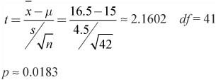
Step 3: With a p-value of 0.0183, we reject the null hypothesis at the 5% level. There appears to be enough evidence to reject the null hypothesis and conclude that the typical teen plays more than 15 hours of video games per week.
![]() Let’s return to the p-value. What does a p-value of 0.0183 really mean? Think about it this way. If the typical teen really does play an average of 15 hours of video games a week, the probability of taking a random sample from that population and obtaining an
Let’s return to the p-value. What does a p-value of 0.0183 really mean? Think about it this way. If the typical teen really does play an average of 15 hours of video games a week, the probability of taking a random sample from that population and obtaining an ![]() value of 16.5 or more is only 0.0183. In other words, it’s possible, but pretty unlikely. Only about 1.83% of the time can we obtain a sample average of 16.5 hours or greater, if the true population mean is 15 hours.
value of 16.5 or more is only 0.0183. In other words, it’s possible, but pretty unlikely. Only about 1.83% of the time can we obtain a sample average of 16.5 hours or greater, if the true population mean is 15 hours.
![]() In Example 2, we rejected the null hypothesis at the 5% level (this is called the alpha level, α). The most common levels at which we reject the null hypothesis are the 5% and 1% levels. That’s not to say that we can’t reject a null hypothesis at the 10% level or even at the 6% or 7% levels; it’s just that 1% and 5% happen to be commonly accepted levels at which we reject or fail to reject the null hypothesis.
In Example 2, we rejected the null hypothesis at the 5% level (this is called the alpha level, α). The most common levels at which we reject the null hypothesis are the 5% and 1% levels. That’s not to say that we can’t reject a null hypothesis at the 10% level or even at the 6% or 7% levels; it’s just that 1% and 5% happen to be commonly accepted levels at which we reject or fail to reject the null hypothesis.
![]() You may struggle a little while first using the p-value to determine whether you should reject or fail to reject the null hypothesis. Always compare your p-value to the given α – level. In Example 2, we used an α – level of 0.05. Our p-value of 0.0183 led us to reject at the 5% level because 0.0183 is less than 0.05. We did not reject at the 1% level because 0.0183 is greater than 0.01. To reject at a given α – level, the p-value must be less than the α – level.
You may struggle a little while first using the p-value to determine whether you should reject or fail to reject the null hypothesis. Always compare your p-value to the given α – level. In Example 2, we used an α – level of 0.05. Our p-value of 0.0183 led us to reject at the 5% level because 0.0183 is less than 0.05. We did not reject at the 1% level because 0.0183 is greater than 0.01. To reject at a given α – level, the p-value must be less than the α – level.
![]() If an α – level is not given, you should use your own judgment. You are probably safe using a 1% or 5% alpha level. However, don’t feel obligated to use a level. You can make a decision based on the p-value without using an alpha level. Just remember that the smaller the p-value, the more evidence you have to reject the null hypothesis.
If an α – level is not given, you should use your own judgment. You are probably safe using a 1% or 5% alpha level. However, don’t feel obligated to use a level. You can make a decision based on the p-value without using an alpha level. Just remember that the smaller the p-value, the more evidence you have to reject the null hypothesis.
![]() The p-value in Example 2 is found by calculating the area to the right of the test statistic t = 2.1602 under the t-distribution with df = 41. If we had used a two-sided alternative instead of a one-sided alternative, we would have obtained a p-value of 0.0367, which would be double that of the one-sided alternative. Thus, the p-value for the two-sided test would be found by calculating the area to the right of t = 2.1602 and combining that with the area to the left of t = −2.1602.
The p-value in Example 2 is found by calculating the area to the right of the test statistic t = 2.1602 under the t-distribution with df = 41. If we had used a two-sided alternative instead of a one-sided alternative, we would have obtained a p-value of 0.0367, which would be double that of the one-sided alternative. Thus, the p-value for the two-sided test would be found by calculating the area to the right of t = 2.1602 and combining that with the area to the left of t = −2.1602.
![]() We are sometimes interested in the difference in two population means, μ1 – μ2. The assumptions and conditions necessary to carry out a confidence interval or test of significance are the same for two-sample means as they are for one-sample means, with the addition that the samples must be independent of one another. You must check the assumptions and conditions for each independent sample.
We are sometimes interested in the difference in two population means, μ1 – μ2. The assumptions and conditions necessary to carry out a confidence interval or test of significance are the same for two-sample means as they are for one-sample means, with the addition that the samples must be independent of one another. You must check the assumptions and conditions for each independent sample.
![]() The assumptions and conditions for a two-sample t-interval or two-sample t-test are as follows:
The assumptions and conditions for a two-sample t-interval or two-sample t-test are as follows:
Assumptions 1. Samples are independent of each other | Conditions 1. Are they? Does this seem reasonable? |
2. Individuals in each sample are independent | 2. Both SRSs and both <10% population (10n<N for both samples) |
3. Normal populations assumption | 3. One of the following:
|
![]() Remember that the mean of the sampling distribution of
Remember that the mean of the sampling distribution of ![]() 1 −
1 − ![]() 2 is μ1 − μ2.
2 is μ1 − μ2.
![]() The standard deviation of the sampling distribution is
The standard deviation of the sampling distribution is 
Remember that the population standard deviations are usually unknown. Recall that when this is the case, we use the sample standard deviation to estimate the population standard deviation. Thus, the standard error (SE) of the sampling distribution is  .
.
![]() Once we’ve checked the assumptions and conditions, we can proceed to finding the confidence interval for the difference of the means of the two independent groups. We can use
Once we’ve checked the assumptions and conditions, we can proceed to finding the confidence interval for the difference of the means of the two independent groups. We can use 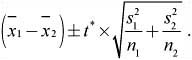
The t* value depends on the particular level of confidence that you want and on the degrees of freedom (df).
![]() To find the degrees of freedom of a two-sample t-statistic, we can use one of two methods:
To find the degrees of freedom of a two-sample t-statistic, we can use one of two methods:
Method 1: Use the calculator-generated degrees of freedom. This gives an accurate approximation of the t-distribution based on degrees of freedom from the data. Usually, we obtain non-whole number values using this method. The formula our calculator uses is somewhat complex, and we probably don’t need to be too concerned with how the degrees of freedom are calculated. Make sure, however, that you always state the degrees of freedom that you are using, regardless of what method you use.
Method 2: Use the degrees of freedom equal to the smaller of the two values of n1 – 1 and n2 – 2. This is considered a conservative method.
![]() Example 3: Two high-school cross-country coaches from different teams are discussing their boys’ and girls’ teams. One coach believes that male and female cross-country runners in the state of Indiana differ in the number of miles they run, on average, each week. The other coach disagrees. He feels that male and female cross-country athletes run about the same number of miles per week, on average. Construct a 95% confidence interval for the difference in average weekly mileage between male and female cross-country runners in the state of Indiana. Consider the data obtained from two independent random samples:
Example 3: Two high-school cross-country coaches from different teams are discussing their boys’ and girls’ teams. One coach believes that male and female cross-country runners in the state of Indiana differ in the number of miles they run, on average, each week. The other coach disagrees. He feels that male and female cross-country athletes run about the same number of miles per week, on average. Construct a 95% confidence interval for the difference in average weekly mileage between male and female cross-country runners in the state of Indiana. Consider the data obtained from two independent random samples:
Boys: 20, 30, 35, 40, 40, 45, 45, 45, 50, 50, 50, 50, 52, 54, 55, 60, 60, 60, 70, 75
Girls: 20, 20, 30, 35, 35, 40, 40, 40, 45, 45, 45, 50, 50, 50, 52, 60, 60, 60, 60, 60
Solution:
Step 1:
Let μ1 = mean weekly mileage for male runners.
Let μ2 = mean weekly mileage for female runners.
Find the mean difference, μ1 − μ2, in weekly mileage between male and female high-school cross-country runners in the state of Indiana.
Assumptions and conditions that verify:
Samples are independent of one another. We are given that the samples are independent of one another.
Individuals are independent. We are given that the samples are random, and we can safely assume that there are more than 200 male and 200 female cross-country runners in the state of Indiana (10n < N for both samples).
Normal population assumption. We are given small samples, but modified boxplots for each sample appear to be symmetric with no outliers. We should be safe using t-procedures.

Step 2: Since the assumptions and conditions have been met, we will construct a two-sample t-interval.
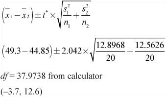
Note that it would also be acceptable to use 19 degrees of freedom, as it is the smaller n−1.
Step 3: We are 95% confident that the true difference in the means of male and female high-school cross-country runners in the state of Indiana is between -3.7 miles and 12.6 miles.
![]() Does our confidence interval shed any light on the coaches’ discussion concerning whether male and female runners differ in weekly average mileage? We can see from our interval that males run between -3.7 miles to 12.6 miles more than their female counterparts. Think about it! What does it mean for male runners to run −3.7 miles more than females? It means that they are running 3.7 miles less than females. Equally important is the fact that zero is contained in the confidence interval, which means that male and female cross-country runners in the state of Indiana might run the same number of weekly miles, on average. Remember, we are not 100% sure of anything. Recall that a 95% confidence interval implies that if we were to construct many, many confidence intervals using the same process, about 95 out of every 100 confidence intervals would contain the true mean difference in the amount of miles run by male and female high-school cross-country runners in the state of Indiana.
Does our confidence interval shed any light on the coaches’ discussion concerning whether male and female runners differ in weekly average mileage? We can see from our interval that males run between -3.7 miles to 12.6 miles more than their female counterparts. Think about it! What does it mean for male runners to run −3.7 miles more than females? It means that they are running 3.7 miles less than females. Equally important is the fact that zero is contained in the confidence interval, which means that male and female cross-country runners in the state of Indiana might run the same number of weekly miles, on average. Remember, we are not 100% sure of anything. Recall that a 95% confidence interval implies that if we were to construct many, many confidence intervals using the same process, about 95 out of every 100 confidence intervals would contain the true mean difference in the amount of miles run by male and female high-school cross-country runners in the state of Indiana.
![]() In the next section, we will perform a two-sample t-test using the same data as the previous problem. We will outline the appropriate steps of inference and then show how the confidence interval relates to the significance test.
In the next section, we will perform a two-sample t-test using the same data as the previous problem. We will outline the appropriate steps of inference and then show how the confidence interval relates to the significance test.
![]() The assumptions and conditions for a two-sample hypothesis test for means are the same as the assumptions and conditions for a two-sample t-interval. The null hypothesis for this type of test can be written as: H0 : μ1 = μ2 or H0 : μ1 − μ2 = 0
The assumptions and conditions for a two-sample hypothesis test for means are the same as the assumptions and conditions for a two-sample t-interval. The null hypothesis for this type of test can be written as: H0 : μ1 = μ2 or H0 : μ1 − μ2 = 0
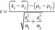
As with a one-sample t-test, the alternative hypothesis can be written with ≠, <, or >. Once the appropriate assumptions and conditions have been met, we can calculate the two-sample t-statistic as follows:
![]() Example 4: Let’s revisit Example 3. Two cross-country coaches from different teams are discussing their boys’ and girls’ teams. One coach believes that male and female cross-country runners in the state of Indiana differ in the number of miles they run, on average, each week. The other coach disagrees. He feels that male and female cross-country athletes run about the same number of miles per week, on average. Is there reason to believe that male and female cross-country runners in Indiana differ in the number of miles they run, on average, each week? Give appropriate statistical evidence to support your answer.
Example 4: Let’s revisit Example 3. Two cross-country coaches from different teams are discussing their boys’ and girls’ teams. One coach believes that male and female cross-country runners in the state of Indiana differ in the number of miles they run, on average, each week. The other coach disagrees. He feels that male and female cross-country athletes run about the same number of miles per week, on average. Is there reason to believe that male and female cross-country runners in Indiana differ in the number of miles they run, on average, each week? Give appropriate statistical evidence to support your answer.
Solution:
Step 1: To answer the question, we will perform a two-sample t-test. We have already defined our variables and checked the appropriate assumptions and conditions for this type of inference in Example 3. We state the null and alternative hypotheses:
H0 : μ1 = μ2
H0 : μ1 ≠ μ2
Step 2: Since the assumptions and conditions have been met, we can calculate the test statistic as follows:
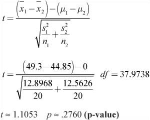
Step 3: With a p-value of approximately 0.2760, we fail to reject the null hypothesis at any reasonable level of significance. We conclude that male and female cross-country runners do not differ in average weekly mileage.
![]() Consider what the p-value really means in this case. If the null hypothesis were really true—that is, male and female cross-country runners in Indiana really do not differ in weekly mileage—the probability of obtaining two samples with average values as different as those obtained is approximately 27.60%. In other words, more than 25% of the time, when sampling, we would obtain sample values from these populations that are as different as or more different than we have obtained. There is not enough statistical evidence to support the claim that males and females differ in weekly average mileage. Remember, typical p-values that lead to rejection of the null hypothesis are usually 10% or less.
Consider what the p-value really means in this case. If the null hypothesis were really true—that is, male and female cross-country runners in Indiana really do not differ in weekly mileage—the probability of obtaining two samples with average values as different as those obtained is approximately 27.60%. In other words, more than 25% of the time, when sampling, we would obtain sample values from these populations that are as different as or more different than we have obtained. There is not enough statistical evidence to support the claim that males and females differ in weekly average mileage. Remember, typical p-values that lead to rejection of the null hypothesis are usually 10% or less.
![]() In the previous section (Example 3), we constructed a 95% confidence interval for the difference in mean weekly mileage between the male and female cross-country runners. Recall that the 95% confidence interval we obtained in Example 3 contained zero. If the difference between μ1 and μ2 were really zero, we could conclude that there was no difference between the means. That is exactly what our results from the significance test in Example 4 are telling us.
In the previous section (Example 3), we constructed a 95% confidence interval for the difference in mean weekly mileage between the male and female cross-country runners. Recall that the 95% confidence interval we obtained in Example 3 contained zero. If the difference between μ1 and μ2 were really zero, we could conclude that there was no difference between the means. That is exactly what our results from the significance test in Example 4 are telling us.
![]() Understand the connection between a confidence interval and a test of significance. A 95% confidence interval is equivalent to a two-sided significance test at the 5% level. A 90% confidence interval is equivalent to a two-sided significance test at the 10% level or to a one-sided test at the 5% level. Make sure you understand the connection between confidence intervals and tests of significance.
Understand the connection between a confidence interval and a test of significance. A 95% confidence interval is equivalent to a two-sided significance test at the 5% level. A 90% confidence interval is equivalent to a two-sided significance test at the 10% level or to a one-sided test at the 5% level. Make sure you understand the connection between confidence intervals and tests of significance.
![]() Recall Example 4 from Chapter 4, concerning a matched-pairs experiment. A manufacturer of bicycle tires wants to test the durability of a new material used in bicycle tires. A completely randomized design might be used where one group of cyclists uses tires made with the “old” material, and another group uses tires made with the “new” material. The manufacturer realizes that not all cyclists will ride their bikes on the same type of terrain and in the same conditions. To help control these variables, we can implement a matched-pairs design. Recall that matching is a form of blocking. One way to do this is to have each cyclist use both types of tires. A coin could be used to determine whether the cyclist uses the tire with the new material on the front of the bike or on the rear. We could then compare the front and rear tires for each cyclist.
Recall Example 4 from Chapter 4, concerning a matched-pairs experiment. A manufacturer of bicycle tires wants to test the durability of a new material used in bicycle tires. A completely randomized design might be used where one group of cyclists uses tires made with the “old” material, and another group uses tires made with the “new” material. The manufacturer realizes that not all cyclists will ride their bikes on the same type of terrain and in the same conditions. To help control these variables, we can implement a matched-pairs design. Recall that matching is a form of blocking. One way to do this is to have each cyclist use both types of tires. A coin could be used to determine whether the cyclist uses the tire with the new material on the front of the bike or on the rear. We could then compare the front and rear tires for each cyclist.
![]() Suppose in this experiment that the researcher has kept track of the number of miles that each tire lasted before needing to be replaced. We might consider looking at the average number of miles that the tires with the new material lasted and compare that with the average number of miles that the tires with the old material lasted. However, we should realize that the assumption of independence has been violated because each cyclist is using one tire with the old material and one tire with the new material. Since the data comes from matching, the data sets are not independent. When this happens, we take the difference for each pair of data and use a one-sample t-procedure, instead of a two-sample t-procedure. Remember: Matched pairs are always a one-sample t-procedure, not a two-sample t-procedure!
Suppose in this experiment that the researcher has kept track of the number of miles that each tire lasted before needing to be replaced. We might consider looking at the average number of miles that the tires with the new material lasted and compare that with the average number of miles that the tires with the old material lasted. However, we should realize that the assumption of independence has been violated because each cyclist is using one tire with the old material and one tire with the new material. Since the data comes from matching, the data sets are not independent. When this happens, we take the difference for each pair of data and use a one-sample t-procedure, instead of a two-sample t-procedure. Remember: Matched pairs are always a one-sample t-procedure, not a two-sample t-procedure!
![]() Example 5: Find a 90% confidence interval for the mean difference in the mileage obtained for tires with the new material and tires with the old material. Following are the paired differences (new minus old) for each of the 17 riders, chosen at random, who took part in the experiment:
Example 5: Find a 90% confidence interval for the mean difference in the mileage obtained for tires with the new material and tires with the old material. Following are the paired differences (new minus old) for each of the 17 riders, chosen at random, who took part in the experiment:
50, 45, 50, 50, 100, 100, 100, -10, 75, -25, 0, 25, 75, 25, 50, 40, 35
Solution:
Step 1: We want to estimate μ, the mean difference in the number of miles obtained from tires using the new material and tires using the old material. It’s common to use μd or μdiff to show that we are interested in the mean difference. Since we are using data from a matched-pairs experiment, we will check the assumptions and conditions for a one sample t-interval.
Assumptions and conditions that verify:
Individuals are independent. We are given that the sample is random. We can safely assume that there are more than 170 cyclists who might use these types of tires (10n < N).
Normal population assumption. We are given a small sample, but a modified boxplot of the differences (Figure 7.5) appears to be fairly symmetric with no outliers. We should be safe using t-procedures.

Step 2: Since the assumptions and conditions are met, we will construct a one-sample t-interval for the differences.

Step 3: We are 90% confident that the mean difference in the number of miles that tires manufactured with the new material lasted compared to those constructed with the old material is between 30.537 and 61.816 miles.
![]() No matter how carefully we set up an experiment or how carefully we obtain a sample, we can always make a mistake when conducting a hypothesis test. Due to sampling variability, we sometimes reject the null hypothesis when we should fail to reject it and sometimes fail to reject the null hypothesis when we should reject it. These types of mistakes are called type I and type II errors.
No matter how carefully we set up an experiment or how carefully we obtain a sample, we can always make a mistake when conducting a hypothesis test. Due to sampling variability, we sometimes reject the null hypothesis when we should fail to reject it and sometimes fail to reject the null hypothesis when we should reject it. These types of mistakes are called type I and type II errors.
A type I error occurs when we reject the null hypothesis when, in fact, it is actually correct. The probability of making a type I error is equal to the significance level (α – level) of the test.
A type II error occurs when we fail to reject the null hypothesis when, in fact, the null hypothesis is false. The probability of a type II error is referred to as β.
![]() Finding the probability of a type I error is as simple as stating the significance level of the test. Students are not responsible for calculating the probability of a type II error, but you should understand the concepts of both type I and type II errors and be able to explain them in context of the problem. You should also understand that the probability of a type II error is dependent upon the chosen alternative value of the given parameter.
Finding the probability of a type I error is as simple as stating the significance level of the test. Students are not responsible for calculating the probability of a type II error, but you should understand the concepts of both type I and type II errors and be able to explain them in context of the problem. You should also understand that the probability of a type II error is dependent upon the chosen alternative value of the given parameter.
![]() The power of the test is the probability of rejecting the null hypothesis given that a particular alternative value is true. The power of the test is equal to 1 − β. We want the power of the test to be relatively high. Think of it this way: If the null hypothesis is not true and a particular alternative value is true, then we should be rejecting the null hypothesis. Typically, we want the power of the test to be around 80% or above.
The power of the test is the probability of rejecting the null hypothesis given that a particular alternative value is true. The power of the test is equal to 1 − β. We want the power of the test to be relatively high. Think of it this way: If the null hypothesis is not true and a particular alternative value is true, then we should be rejecting the null hypothesis. Typically, we want the power of the test to be around 80% or above.
![]() There are four ways we can increase the power of a hypothesis test. The first two are probably the most important for you to remember.
There are four ways we can increase the power of a hypothesis test. The first two are probably the most important for you to remember.
Increase the a – level. Increasing the α – level is one method of increasing the power of the test.
Increase the sample size. Increasing the sample size makes us more confident about our decision to reject or fail to reject the null hypothesis. Cost sometimes prohibits increasing the sample size.
Decrease the standard deviation. Sometimes it is possible to decrease the standard deviation, and sometimes it is not. Machinery can sometimes be finely tuned so that the production of goods can be more precise, which can in turn reduce the variability.
Choose a different alternative value. Choosing an alternative value that is further away from the value of the null hypothesis will increase the value of the power. The power is affected by the difference between the hypothesized value and the true value of the parameter.