8.1 One-Sample z-Interval for Proportions
8.2 One-Sample z-Test for Proportions
8.3 Two-Sample z-Interval for Difference Between Two Proportions
8.4 Two-Sample z-Test for Difference Between Two Proportions
![]() Now that we’ve discussed various statistical inference procedures for population means, it’s time to turn our attention to statistical inference involving proportions. We are often concerned about the unknown proportion of the population that has some particular outcome of interest.
Now that we’ve discussed various statistical inference procedures for population means, it’s time to turn our attention to statistical inference involving proportions. We are often concerned about the unknown proportion of the population that has some particular outcome of interest.
![]() Remember the appropriate statistical notation when dealing with proportions. Always use
Remember the appropriate statistical notation when dealing with proportions. Always use ![]() when referring to a sample proportion and p when referring to a population proportion.
when referring to a sample proportion and p when referring to a population proportion.
![]() As discussed in Chapter 6, the sampling distribution of
As discussed in Chapter 6, the sampling distribution of ![]() is approximately normal, provided that np and n(1 − p) are at least 10. The standard deviation of the sampling distribution of
is approximately normal, provided that np and n(1 − p) are at least 10. The standard deviation of the sampling distribution of ![]() is
is  as long as the population is at least 10 times the sample size. When dealing with confidence intervals, we do not know p. Because
 ![]() is an unbiased estimator of p, we use
is an unbiased estimator of p, we use ![]() to estimate p. These two values should be close in value, provided that the sample is large enough. We can then use the standard error of
to estimate p. These two values should be close in value, provided that the sample is large enough. We can then use the standard error of ![]() , which is:
, which is: 
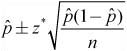
![]() When constructing a one-proportion z-interval, we use:
When constructing a one-proportion z-interval, we use:
![]() As with any type of inference, always check the assumptions and conditions of the inference procedure. The assumptions and conditions for a one-proportion z-interval or test are:
As with any type of inference, always check the assumptions and conditions of the inference procedure. The assumptions and conditions for a one-proportion z-interval or test are:
Assumptions 1. Individuals are independent | Conditions 1. SRS and n < 10% of population |
2. Sample is large enough | 2. np ≥ 10 and n(1 − p) ≥ 10 Use |
![]() To ensure that we include all the essentials of inference, we will follow the 3-step method used in Chapter 7.
To ensure that we include all the essentials of inference, we will follow the 3-step method used in Chapter 7.
Identify the parameter of interest, choose the appropriate inference procedure, and verify that the assumptions and conditions for that procedure are met.
Carry out the inference procedure. Do the math! Be sure to apply the correct formula.
Interpret the results in context of the problem.
![]() Example 1: Cassidy is interested in knowing the percentage of fourth graders in the Indianapolis area who own a cell phone in hopes of convincing her parents that she should own one too. With the help of her favorite statistician, she gathers information from a random sample of 100 fourth graders in the Indianapolis area. She finds that 18 of the 100 fourth graders sampled do indeed own a cell phone. Construct a 90% confidence interval for the true proportion of fourth graders who own cell phones.
Example 1: Cassidy is interested in knowing the percentage of fourth graders in the Indianapolis area who own a cell phone in hopes of convincing her parents that she should own one too. With the help of her favorite statistician, she gathers information from a random sample of 100 fourth graders in the Indianapolis area. She finds that 18 of the 100 fourth graders sampled do indeed own a cell phone. Construct a 90% confidence interval for the true proportion of fourth graders who own cell phones.
Solution:
Step 1: We want to estimate p, the true proportion of fourth graders who own cell phones. We must check the assumptions and conditions.
Assumptions and conditions that verify:
Individuals are independent. We are given a random sample, and we are safe to assume that there are more than 1000 fourth graders in the Indianapolis area (10n<N).
Sample is large enough:
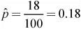
100(.18) = 18 ≥ 10 and 100(.82) = 82 ≥ 10. Hence, we are safe to assume that the sampling distribution of
 is approximately normal.
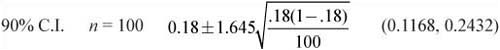
Step 2: Since the assumptions and conditions for inference have been met, we will construct the one-proportion z-interval.

Step 3: We are 90% confident that the true proportion of fourth graders who own cell phones in the Indianapolis area is between 11.68% and 24.32%. Cassidy will remain one of those “unfortunate” fourth graders who do not own a cell phone.
![]() Now that we’ve discussed how to construct a one-sample t-interval for the mean of a population and a one-proportion z-interval for the population proportion, it’s time to discuss the margin of error. When dealing with a one-proportion z-interval, the margin of error is the distance from the endpoints of the confidence interval to the center of the interval,
Now that we’ve discussed how to construct a one-sample t-interval for the mean of a population and a one-proportion z-interval for the population proportion, it’s time to discuss the margin of error. When dealing with a one-proportion z-interval, the margin of error is the distance from the endpoints of the confidence interval to the center of the interval, ![]() . The margin of error is the product of the z* value and the standard error and is affected primarily by the sample size and the z* value (confidence level). The margin of error for a t-interval is affected in a similar fashion by the sample size and the level of confidence.
. The margin of error is the product of the z* value and the standard error and is affected primarily by the sample size and the z* value (confidence level). The margin of error for a t-interval is affected in a similar fashion by the sample size and the level of confidence.
![]() We know that as the sample size increases, the variability of the sampling distribution decreases. The effects of changing the sample size on the confidence interval become evident if we change the sample size while keeping the standard deviation and confidence level the same. Consider Example 1: How does the confidence interval change when we increase the sample size in Example 1 from 100 to 500? What happens if we increase the sample size in Example 1 to 1000?
We know that as the sample size increases, the variability of the sampling distribution decreases. The effects of changing the sample size on the confidence interval become evident if we change the sample size while keeping the standard deviation and confidence level the same. Consider Example 1: How does the confidence interval change when we increase the sample size in Example 1 from 100 to 500? What happens if we increase the sample size in Example 1 to 1000?

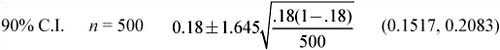
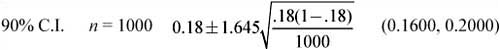
Notice that as the sample size increases, the width of the confidence interval decreases. This is due to the fact that there is less sampling variability in larger samples than in smaller samples. Thus, the standard deviation of the sampling distribution is smaller, and, consequently, the margin of error is smaller. This causes the confidence interval to be narrower. It’s easy to see the advantage of using larger samples when performing inference. Cost and other factors sometimes prohibit using larger samples.
![]() What about the level of confidence for the interval? How does the confidence interval in Example 1 change if we keep the sample size of 100 but change the level of confidence to 95%? What happens to the confidence interval if we change the level of confidence to 99%?
What about the level of confidence for the interval? How does the confidence interval in Example 1 change if we keep the sample size of 100 but change the level of confidence to 95%? What happens to the confidence interval if we change the level of confidence to 99%?
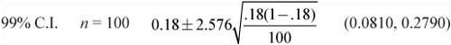

Notice that as the confidence level increases, so does the width of the confidence interval. Mathematically, this is the result of using a different value for z*. Recall that z* is the number of standard deviations from the mean. To be more confident that our interval contains the true population proportion, the interval must be wider. Realize that the cost of increasing the level of confidence is that the interval becomes wider as the level increases.
![]() We are sometimes required to find the sample size needed to obtain a desired margin of error. The next example illustrates how to find the needed sample size when dealing with proportions. A similar method is used to find the sample size when dealing with means.
We are sometimes required to find the sample size needed to obtain a desired margin of error. The next example illustrates how to find the needed sample size when dealing with proportions. A similar method is used to find the sample size when dealing with means.
![]() Example 2: A polling organization wants to determine the sample size needed to estimate p, the proportion of voters who plan to vote for a particular candidate. The organization wants to estimate p with 98% confidence and a margin of error of no more than 3%. How large of a sample is needed?
Example 2: A polling organization wants to determine the sample size needed to estimate p, the proportion of voters who plan to vote for a particular candidate. The organization wants to estimate p with 98% confidence and a margin of error of no more than 3%. How large of a sample is needed?
Solution: We can use the formula for the margin of error.

Using 2.326 (98% confidence) for z and 0.5 for p*
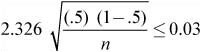
Solving for n, we obtain:
n ≥ 1502.8544
Because the number of people surveyed must be a whole number, we round to 1503. It should be noted that 0.5 is used for p*. If previous sampling had been done and an estimate of p had been obtained, that estimate could be used instead of 0.5. However, 0.5 will always give a sample size that is larger than any other value used for p*. So if in doubt, use 0.5.
![]() As mentioned earlier, we can find a desired sample size needed for a particular margin of error when dealing with means in the same manner as we do proportions. Just use the part of the formula that comes after the ± in the appropriate confidence interval and solve for n. Always round your answer up to the next whole number.
As mentioned earlier, we can find a desired sample size needed for a particular margin of error when dealing with means in the same manner as we do proportions. Just use the part of the formula that comes after the ± in the appropriate confidence interval and solve for n. Always round your answer up to the next whole number.
![]() Hypothesis testing for a one-proportion z-test is similar to that of a one-sample t-test, at least to some extent. The difference is that we are dealing with proportions instead of means. The assumptions and conditions are the same for a one-proportion z-test as they are for a one-proportion z-interval. Keep in mind, however, that since we do not know the true population proportion, p, we use the hypothesized value, p0, when checking the assumptions and conditions. We also use p0 for calculating the standard error of the sampling distribution of
Hypothesis testing for a one-proportion z-test is similar to that of a one-sample t-test, at least to some extent. The difference is that we are dealing with proportions instead of means. The assumptions and conditions are the same for a one-proportion z-test as they are for a one-proportion z-interval. Keep in mind, however, that since we do not know the true population proportion, p, we use the hypothesized value, p0, when checking the assumptions and conditions. We also use p0 for calculating the standard error of the sampling distribution of ![]() . As with a one-sample t-test, we use an equality when stating the null hypothesis and an inequality when stating the alternative hypothesis. We will use the same three-step process for organizing the inference procedure as we have done thus far to help ensure that we include the essentials of inference.
. As with a one-sample t-test, we use an equality when stating the null hypothesis and an inequality when stating the alternative hypothesis. We will use the same three-step process for organizing the inference procedure as we have done thus far to help ensure that we include the essentials of inference.
![]() Provided that the assumptions and conditions for a one-proportion z-test are met, we can calculate the test statistic using:
Provided that the assumptions and conditions for a one-proportion z-test are met, we can calculate the test statistic using:
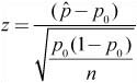
We then obtain a p-value based on the value of z and make a decision whether to reject or fail to reject the null hypothesis. Consider the following example.
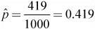
![]() Example 3: A beverage company claims that 45% of adults drink diet soda. Skeptical about the claim, Addison obtains a random sample of 1000 adults and finds that 419 of them drink diet soda. Is there evidence to support Addison's suspicion that less than 45% of adults drink diet soda?
Example 3: A beverage company claims that 45% of adults drink diet soda. Skeptical about the claim, Addison obtains a random sample of 1000 adults and finds that 419 of them drink diet soda. Is there evidence to support Addison's suspicion that less than 45% of adults drink diet soda?
Solution:
Step 1: We will conduct a one-proportion z-test.
Let p = proportion of all adults who drink diet soda
H0 : p = 0.45
Ha : p < 0.45
Assumptions and conditions that verify:
Individuals are independent. We are given a random sample, and we are safe to assume that there are more than 10,000 adults who drink diet soda (10n<N).
Sample is large enough:
1000(.419) = 419 ≥ 10 and 1000(.581) = 581 ≥ 10. Be sure to show the actual numbers! Therefore, we are safe to assume that the sampling distribution of
is approximately normal.
Step 2: The assumptions and conditions for inference have been met; we will perform a one-proportion z-test.

Step 3: With a p-value of 0.0244, we reject the null hypothesis at the 5% level. We conclude that the proportion of adults who drink diet soda is less then 45%.
![]() Remember, a p-value of 0.0244 would allow us to reject the null hypothesis at the 5% level, but not at the 1% level. A sample
Remember, a p-value of 0.0244 would allow us to reject the null hypothesis at the 5% level, but not at the 1% level. A sample ![]() value of 0.419 or less would occur only about 2.44% of the time, purely due to chance, if the true proportion of all adults who drank diet soda really were 45%. This gives us evidence to reject the null hypothesis at the 5% level.
value of 0.419 or less would occur only about 2.44% of the time, purely due to chance, if the true proportion of all adults who drank diet soda really were 45%. This gives us evidence to reject the null hypothesis at the 5% level.
![]() We are sometimes interested in comparing the proportion of successes between two groups. For example, we might be interested in knowing the difference in the proportion of males and females who text while driving. Or, we might be interested in the difference between the portion of college and high-school students who use laptops on a regular basis in their classes.
We are sometimes interested in comparing the proportion of successes between two groups. For example, we might be interested in knowing the difference in the proportion of males and females who text while driving. Or, we might be interested in the difference between the portion of college and high-school students who use laptops on a regular basis in their classes.
![]() We use the statistic
We use the statistic ![]() 1 −
1 − ![]() 2 to estimate the true difference in the population proportions, p1 – p2. Remember that
2 to estimate the true difference in the population proportions, p1 – p2. Remember that ![]() 1 −
1 − ![]() 2 is an unbiased estimator of p1 – p2.
2 is an unbiased estimator of p1 – p2.
![]() The standard deviation of the sampling distribution of
The standard deviation of the sampling distribution of ![]() 1 −
1 − ![]() 2 is
2 is 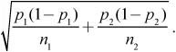
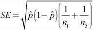
When dealing with a confidence interval, the values of p1 and p2 are unknown. For this reason, we use the standard error of the statistic ![]() 1 −
1 − ![]() 2:
2:

![]() The formula for the confidence interval for comparing two proportions is:
The formula for the confidence interval for comparing two proportions is:

![]() The assumptions and conditions for inference when working with two proportions are as follows:
The assumptions and conditions for inference when working with two proportions are as follows:
Assumptions 1. Samples are independent of each other | Conditions 1. Is this reasonable? |
2. Individuals in each sample are independent | 2. Both samples are SRSs and n<10% of population for both samples |
3. Both samples are large enough | 3. np≥ 10 and n(1 – p) ≥ 10 for both samples |
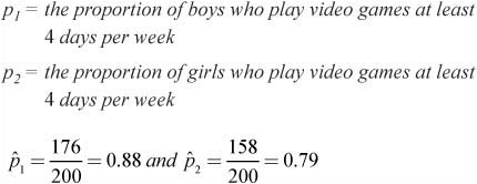
![]() Example 4: Nolan hopes to determine the difference in the proportion of males and females who play video games at least 4 days per week. Two independent random samples of size 200 are obtained. Of the 200 girls surveyed, 158 play video games at least 4 days per week. Of the 200 boys surveyed, 176 play video games at least 4 days per week. Construct a 99% confidence interval to help answer Nolan’s question.
Example 4: Nolan hopes to determine the difference in the proportion of males and females who play video games at least 4 days per week. Two independent random samples of size 200 are obtained. Of the 200 girls surveyed, 158 play video games at least 4 days per week. Of the 200 boys surveyed, 176 play video games at least 4 days per week. Construct a 99% confidence interval to help answer Nolan’s question.
Solution:
Step 1: We want to estimate p1 – p2.
Assumptions and conditions that verify:
Samples are independent of each other. We are given that the samples are independent of one another.
Individuals in each sample are independent. Both samples are given to be random, and we can safely assume that there are more than 2000 boys and 2000 girls in the population (10n<N for both samples).
Both samples are large enough: 200(0.88) ≥ 10 and 200(0.12) ≥ 10.
200(0.79) ≥ 10 and 200(0.21) ≥ 10.
Step 2: The assumptions and conditions are met; we are safe to construct a two-proportion z-interval.
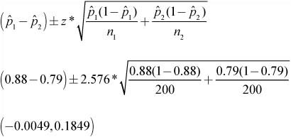
Step 3: We are 99% confident that the true difference in the proportion of boys and girls who play video games at least 4 days per week is between –.49% and 18.49%.
![]() Keep in mind that the interval contains zero. This means that zero is a plausible value for the difference in the proportion of boys and girls who play video games at least 4 days per week. Zero is contained in the interval, and we are 99% confident that the true difference is captured in the confidence interval that we have obtained. Note that a 95% confidence interval (0.00429, 0.17571) does not contain zero.
Keep in mind that the interval contains zero. This means that zero is a plausible value for the difference in the proportion of boys and girls who play video games at least 4 days per week. Zero is contained in the interval, and we are 99% confident that the true difference is captured in the confidence interval that we have obtained. Note that a 95% confidence interval (0.00429, 0.17571) does not contain zero.
![]() We are sometimes interested in knowing whether or not two population proportions are really different from one another. Remember that when sampling, we always encounter sampling variability. When we find the sample proportions, we want to determine if there really is a difference between the population proportions or if the difference between the obtained sample proportions is purely due to chance.
We are sometimes interested in knowing whether or not two population proportions are really different from one another. Remember that when sampling, we always encounter sampling variability. When we find the sample proportions, we want to determine if there really is a difference between the population proportions or if the difference between the obtained sample proportions is purely due to chance.
![]() The null hypothesis for a two-proportion z-test is H0 : p1 = p2. The alternative hypothesis can be one- or two-sided. To conduct the hypothesis test, we need to standardize the test statistic,
The null hypothesis for a two-proportion z-test is H0 : p1 = p2. The alternative hypothesis can be one- or two-sided. To conduct the hypothesis test, we need to standardize the test statistic, ![]() 1 −
1 − ![]() 2. If the null hypothesis is true, then the observations from each sample actually belong to a singe population. Therefore, instead of estimating each sample proportion separately, we use the pooled sample proportion. To find the pooled sample proportion, we use:
2. If the null hypothesis is true, then the observations from each sample actually belong to a singe population. Therefore, instead of estimating each sample proportion separately, we use the pooled sample proportion. To find the pooled sample proportion, we use:
![]() Once the pooled sample proportion is calculated, we can then find the standard error of the sampling distribution. Recall that for the two-proportion z-interval, we used:
Once the pooled sample proportion is calculated, we can then find the standard error of the sampling distribution. Recall that for the two-proportion z-interval, we used:

Replacing each sample proportion with the pooled proportion, we obtain:

We can simplify the standard error to obtain:
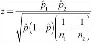
![]() The assumptions and conditions for inference for a two-proportion z-test are the same as those for a two-proportion z-interval. Provided the assumptions and conditions for inference are met, we can use the test statistic:
The assumptions and conditions for inference for a two-proportion z-test are the same as those for a two-proportion z-interval. Provided the assumptions and conditions for inference are met, we can use the test statistic:
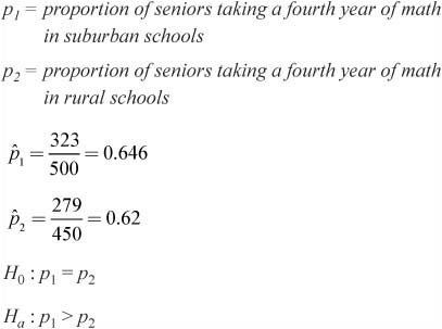
![]() Example 5: A local college is interested in knowing if the proportion of high school students taking a fourth year of math is greater for students in suburban schools than in rural schools. To help answer this question, the college obtains a random sample of 500 senior students from suburban school districts and a random sample of 450 senior students from rural school districts across the country. The survey reveals that, of the 500 suburban students, 323 are taking a fourth year of math while only 279 of the 450 rural students are taking a fourth year of math. Is there evidence to suggest that the proportion of seniors taking a fourth year of math in suburban school districts is greater than the proportion of seniors taking a fourth year of math in rural school districts at the 5% level?
Example 5: A local college is interested in knowing if the proportion of high school students taking a fourth year of math is greater for students in suburban schools than in rural schools. To help answer this question, the college obtains a random sample of 500 senior students from suburban school districts and a random sample of 450 senior students from rural school districts across the country. The survey reveals that, of the 500 suburban students, 323 are taking a fourth year of math while only 279 of the 450 rural students are taking a fourth year of math. Is there evidence to suggest that the proportion of seniors taking a fourth year of math in suburban school districts is greater than the proportion of seniors taking a fourth year of math in rural school districts at the 5% level?
Step 1:
Assumptions and conditions that verify:
Samples are independent of each other. We can assume that the samples are independent of one another because they are taken from school districts in different areas.
Individuals in each sample are independent. Both samples are given to be random, and we can safely assume that there are more than 5000 seniors in suburban school districts and 4500 seniors in rural school districts (10n<N for both samples).
Both samples are large enough: 500(0.646) ≥ 10 and 500(0.354) ≥ 10.
450(0.62) ≥ 10 and 200(0.38) ≥ 10.
Step 2: Because the assumptions and conditions for inference have been met, we should be safe to perform a two-sample z-test.

Step 3: With a p-value of 0.2031, we fail to reject the null hypothesis at the 5% level. We conclude that the proportion of seniors taking a fourth year of math in suburban schools is not greater than the proportion of seniors taking a fourth year of math in rural schools.