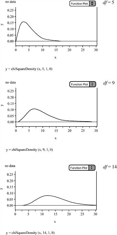
When our inference procedures involve categorical variables and our data are given in the form of counts, we turn to the chi-square statistic (χ²). The chi-square statistic is actually a family of distributions and is always skewed to the right. Each of these distributions is classified by its degrees of freedom. Like the t-distributions, the distribution changes shape based on the degrees of freedom. As the degrees of freedom increase, the chi-square distributions become less skewed and become more symmetrical and more normal, as seen in Figure 9.1. All chi-square density curves start at zero on the x-axis, are single peaked, and approach the x-axis, asymptotically, as x increases (except when df = 1).

The chi-square test statistic can be found using:

where O is the observed count and E is the expected count.

We will discuss three types of tests involving the chi-square distributions. These include: Chi-Square Test for Goodness of Fit, Chi-Square Test for Homogeneity of Populations, and the Chi-Square Test of Association/ Independence. All three of these tests involve finding the same test statistic. We can find the p-value of each test by calculating the area under the chi-square distribution to the right of the test statistic. Remember that, like any density curve, the area under the chi-square distribution is equal to one.

Figure 9.1. Chi-square distributions with 5, 9, and 14 degrees of freedom.

When performing chi-square tests of significance, we will use the familiar three-step format that we have used for all inference procedures. Again, there’s nothing magical about the three steps; it’s just a system you can use to ensure that you are always including the essentials of inference and that you are doing so in an organized fashion. The outline of the three steps is as follows:

We sometimes want to examine the proportions in a single population. In this case, we turn to the Chi-Square Test for Goodness of Fit. You may have used or seen the chi-square test for goodness of fit in your biology class, for it is often used in the field of genetics. The goodness of fit test can be used by scientists to determine whether their hypothesized ratios are indeed correct. The null hypothesis in a goodness of fit test is that the actual population proportions are equal to the hypothesized values. The alternative hypothesis is that the actual population proportions are different from the hypothesized values.

We can use the goodness of fit test to determine how well the observed counts match the expected counts. A classic example of the goodness of fit test is the M&M’s candy activity. In this activity, we want to determine whether the M&M’s candies are really manufactured in the proportions claimed by the manufacturer. This activity will help you understand when to use the goodness of fit test and how the goodness of fit test works. It could be implemented with any type of M&M’s candies as long as you know the claimed proportions for each color. Skittles or any other type of candy or cereal could also be used provided you know the claimed proportions for each color. We will use this activity in Example 1 to perform a goodness of fit test.

As with all inference, we must be sure to check the assumptions and conditions of the test. Following are the assumptions and conditions for the chi-square goodness of fit test:

Once we have checked the assumptions and conditions for inference, we can calculate the chi-square test statistic to test the hypothesis of either a uniform distribution for the given categories or some specified distribution for each category. We can use the test statistic:

The chi-square statistic for a goodness of fit test has n−1 degrees of freedom, where n is the number of categories(not the sample size).

We can calculate the p-value of the test by looking up the critical value with the correct degrees of freedom in the chi-square table of values or by using the graphing calculator χ² cdf command. We will discuss how to use the table of chi-square values in Example 1.

Example 1: Mars Candy claims that plain M&M’s candies are manufactured in the following proportions: 13% brown and red, 14% yellow, 24% blue, 20% orange, and 16% green. Using a 1.69-ounce bag of plain M&M’s, test the manufacturer’s claim at the 5% level of significance. For this example, we will use the following counts obtained from a 1.69-ounce bag of plain M&M’s. We can find the expected number for each color by multiplying the total number of M&M’s in the bag by the claimed proportion for each color. There were 56 M&M’s in the bag. Figure 9.2 contains the observed counts as well as the expected counts for each of the six different colors. The expected counts for each color can be found by multiplying 56 (the total number of M&M’s in the bag) by the corresponding claimed proportion for each color.

Solution:

Step 1: We will use a chi-square goodness of fit test to test the manufacturer’s claim for the proportion of brown, red, yellow, orange, green, and blue M&M’s.

Assumptions and conditions that verify:

Step 2: With the assumptions and conditions of inference met, we should be safe to conduct a chi-square goodness of fit test. We find the test statistic using:

Step 3: With a p-value of approximately 0.7244, we fail to reject the null hypothesis at the 5% level of significance. We conclude that the proportions of colors of M&M’s candies are not different from the proportions claimed by the manufacturer.

In step 2, we obtained a p-value of 0.7244. We can interpret the p-value to mean the following: If repeated samples were taken (that is, many different bags of M&M’s), we would anticipate observed counts as different or more different from the expected counts as we have obtained about 72% of the time, given that the claimed proportions by the manufacturer are really true. In other words, it’s quite likely that the difference we are observing between the observed counts and expected counts is really just due to chance (sampling variability).

How do we obtain the p-value of 0.7244? There are two methods, as mentioned earlier in this chapter. The first method is to use the χ² table of values to approximate the p-value. Remember that we are testing the manufacturer’s claim at the 5% level. To use the table, we need to determine the critical value. The critical value is based, in part, by the level of significance at which we want to test our claim, and in part to the degrees of freedom. Using the χ² table of values, we can locate the critical value by cross-referencing 0.05 at the top of the table with 5 degrees of freedom. The corresponding critical value is 11.07. If we obtain a χ² test statistic greater than the critical value of 11.07, then we know that the corresponding p-value would be less than 0.05, which would lead us to reject the null hypothesis. Because our χ² value was only 2.8415, which is less than 11.07, we know the p-value is greater than 0.05. In fact, if we examine the table a little more closely, we can see that the smallest critical value for 5 degrees of freedom is 6.63. Our χ² value of 2.8415 is smaller than 6.63. We can therefore conclude that the p-value for our test will be greater than .25. Thus, we fail to reject the null hypothesis at the 5% level of significance. Using the critical value to estimate the p-value can also be used when working with t-distributions. Typically, we use our calculators to find the p-value by performing the appropriate test command.

The second and most common way of finding the p-value for a chi-square goodness of fit test is to use the graphing calculator. Some graphing calculators have the goodness of fit test built into them. This makes it easy to find both the test statistic and the p-value. Some TI calculators have this test; others do not. Because some do not, we will briefly describe how to obtain the p-value for the goodness of fit test when the test is not built into the calculator.

The TI-83 and TI-84 are both capable of creating lists. Place the observed values in List 1 and the expected values in List 2. Define List 3 to be

We can then use the sum command, which is found under 2^nd STAT (LIST), MATH. The value obtained for the sum of List 3 is the test statistic. We then use the command 2^nd VARS (DISTR) and use the χ² command to determine the p-value.

In Chapter 8, we discussed how to compare two proportions from two different groups using two-proportion z-procedures. We sometimes need to compare proportions across multiple groups. When we want to know if category proportions are the same for each group, we use the Chi-Square Test for Homogeneity. The data typically appear in two-way tables, as there are sometimes several categories. The chi-square test of homogeneity of populations eliminates the problem of comparing proportion 1 to proportion 2, proportion 1 to proportion 3, proportion 2 to proportion 3, and so on, as would be the case using multiple z-proportions.

Although we are trying to determine whether the proportions for multiple populations are the same, it’s important to remember that we are still working with counts. The expected counts for a chi-square test of homogeneity are not found in the same manner as they are in a goodness of fit test. To find the expected counts for a chi-square test of homogeneity, we use the following:

The degrees of freedom are also calculated differently in a chi-square test of homogeneity than they are for a goodness of fit test. To find the degrees of freedom for a chi-square test of homogeneity, we use the following:

The null hypothesis for a chi-square test of homogeneity is that the distribution (proportion) of the counts for each group is the same. The alternative hypothesis is that the distribution for the counts for each group is not the same. We can write the null and alternative hypotheses in words or symbols.

Because we are working with observed and expected counts, the chi-square test for homogeneity uses the same test statistic as the goodness of fit test.

As is the case for all inference procedures, we must always check the assumptions and conditions. The assumptions and conditions for a chi-square test of homogeneity are:

Consider the following hypothetical example involving the comparison of three proportions from three different populations.

Example 2: A group of physicians specializing in weight loss is interested in knowing whether appetite suppressants are effective in helping people lose weight. They are curious to know if they should recommend regular exercise, appetite suppressants, or both to their patients. Suppose that a controlled experiment were conducted yielding the following results (see Figure 9.3). We will consider the proportion of those who lose at least 10 lbs. in a four-week period of time to be a success.

Solution:

Step 1: We want to compare the proportions of patients who lost at least 10 lbs. in a four-week period in the populations of patients who used exercise only (p₁), did not exercise but took an appetite suppressant (p₂), exercised and took the suppressant (p₃), exercised and took a placebo (p₄), and took a placebo only (p₅). We will use a chi-square test for homogeneity of populations.

Assumption and conditions that verify:

Step 2: With the assumptions and conditions met, we will conduct a chi-square test for homogeneity of populations. We can find the test statistic using:

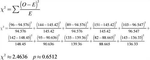
Step 3: With a p-value of 0.6512, we fail to reject the null hypothesis. We conclude that there is not a difference in the proportions of patients who would lose at least 10 lbs. in a four-week period in the populations of patients who: exercise only (p₁), do not exercise but take an appetite suppressant (p₂), exercise and take the suppressant (p₃), exercise and take a placebo (p₄), and take a placebo only (p₅). The appetite suppressant does not appear to help patients lose weight.

We use a Chi-Square Test for Independence/Association to determine whether there is an association between two categorical variables in a single population. As with the chi-square test for homogeneity, the data are usually given in two-way tables. When testing for independence/ association, the two-way tables are called contingency tables because we are classifying individuals into two categorical variables.

When do you use a chi-square test of homogeneity, and when do you use a chi-square test for independence/association? In order to differentiate between the two types of tests, you need to think about the design of the study.

Remember that in a test of independence/association, there is a single sample from a single population. The individuals within the samples are classified according to two categorical variables. The chi-square test for homogeneity, on the other hand, takes only one sample from each of the populations of interest. Each individual from the sample is categorized based on a single variable. Thus, the null and alternative hypotheses differ depending on how the study was designed.

The null hypothesis for a chi-square test of association/independence is that there is no relationship between the two categorical variables of interest. The alternative hypothesis is that there is a relationship between the two categorical variables of interest. We typically write the null and alternative in one of the following two ways:

We will use the same three-step procedure we have used for all inferences thus far, including the assumptions and conditions for the chi-square test for independence/association. The assumptions and conditions for this test are:

Since the data are in counts, we continue to use the same chi-square test statistic:

Example 3: You wish to evaluate the association between a person’s gender and attitude toward spending money on public education. You obtain a random sample from your community and construct the contingency table shown in Figure 9.4.

Is there a relationship between gender and attitudes toward educational spending? Conduct an appropriate test to answer this question.

Solution:

Step 1: We are interested in knowing whether there is an association between a person’s gender and attitude toward spending money on public education. We have obtained a single sample from a single population, so we will conduct a chi-square test for association/ independence. The null and alternative hypotheses are:

We can check the appropriate assumptions and conditions.

Assumption and conditions that verify:

Step 2: We have verified the conditions for inference for a chi-square test of association/independence. We are safe to find the chi-square test statistic:

Step 3: With a p-value of 0.0322, we reject the null hypothesis. There appears to be significant evidence (small p-value) to suggest that there is an association between a person’s gender and attitudes toward spending money on public education.