10.2 Confidence Intervals for the Slope β
10.3 Hypothesis Testing for the Slope β
![]() Inference for regression is the final type of inference discussed in AP Statistics. We use inference for regression when dealing with two quantitative variables. In Chapter 2, we discussed how to model data by using linear, exponential, and power functions. This chapter focuses on how to create confidence intervals for the slope of the least-squares regression line, ŷ = a + bx. You will also learn how to perform a hypothesis test for the slope of a linear relationship.
Inference for regression is the final type of inference discussed in AP Statistics. We use inference for regression when dealing with two quantitative variables. In Chapter 2, we discussed how to model data by using linear, exponential, and power functions. This chapter focuses on how to create confidence intervals for the slope of the least-squares regression line, ŷ = a + bx. You will also learn how to perform a hypothesis test for the slope of a linear relationship.
![]() In Chapter 2, we created the least-squares regression line, ŷ = a + bx from the sample data collected from the population. As such, the slope b, and the y-intercept a, are statistics, not parameters. Remember that, due to sampling variability, the statistics a and b would probably take on different values if we took multiple samples. In other words, if another sample were taken, different data points would produce a different least-squares regression line and, consequently, different values of a and b. Recall that the least-squares regression line is formed by making the sum of the squares of the residuals as small as possible. Also remember that a residual is the difference in the observed value and the predicted value of y.
In Chapter 2, we created the least-squares regression line, ŷ = a + bx from the sample data collected from the population. As such, the slope b, and the y-intercept a, are statistics, not parameters. Remember that, due to sampling variability, the statistics a and b would probably take on different values if we took multiple samples. In other words, if another sample were taken, different data points would produce a different least-squares regression line and, consequently, different values of a and b. Recall that the least-squares regression line is formed by making the sum of the squares of the residuals as small as possible. Also remember that a residual is the difference in the observed value and the predicted value of y.
residual = observed y – predicted y = y – ŷ
![]() Remember that we use the least-squares regression line to make predictions of the response variable, y, based on the explanatory variable, x. We will use the statistics a and b as unbiased estimates of the true slope and y-intercept, which are the unknown parameters, α and β. The mean, μy of all responses has a linear relationship with x that represents the true regression line where:
Remember that we use the least-squares regression line to make predictions of the response variable, y, based on the explanatory variable, x. We will use the statistics a and b as unbiased estimates of the true slope and y-intercept, which are the unknown parameters, α and β. The mean, μy of all responses has a linear relationship with x that represents the true regression line where:
μy = α + βx
![]() Now that we’ve discussed how to estimate the slope and y-intercept of the true regression line, it’s time to discuss the third parameter of interest in inference for regression, the standard deviation, σ. The standard deviation, σ, is used to measure the variability of the response variable y about the true regression line. Remember that the predicted values, ŷ, are on the regression line. The observed values of y vary about the regression line for any given value of x.
Now that we’ve discussed how to estimate the slope and y-intercept of the true regression line, it’s time to discuss the third parameter of interest in inference for regression, the standard deviation, σ. The standard deviation, σ, is used to measure the variability of the response variable y about the true regression line. Remember that the predicted values, ŷ, are on the regression line. The observed values of y vary about the regression line for any given value of x.
![]() If we are given n data points, there will be n residuals. Since σ is the standard deviation of the responses about the true regression line, we estimate σ by using the standard deviation of the residuals of the sample data. Because we are using an estimate for σ, we call the standard deviation the standard error as we have done in previous chapters. We refer to the standard deviation of the response variable as s.
If we are given n data points, there will be n residuals. Since σ is the standard deviation of the responses about the true regression line, we estimate σ by using the standard deviation of the residuals of the sample data. Because we are using an estimate for σ, we call the standard deviation the standard error as we have done in previous chapters. We refer to the standard deviation of the response variable as s.
![]() The standard error about the regression line is:
The standard error about the regression line is:
or


![]() Typically, we use our calculators to find the value of s. In some problems, the value of s will be given.
Typically, we use our calculators to find the value of s. In some problems, the value of s will be given.
![]() Notice that the formula for the standard deviation involves averaging the squared residuals (deviations) from the line. When we find the average of these squared deviations, we are dividing by n − 2. Because we are working with two variables, we use n – 2 degrees of freedom instead of n – 1 degrees of freedom. Be sure to state the degrees of freedom when performing inference for regression.
Notice that the formula for the standard deviation involves averaging the squared residuals (deviations) from the line. When we find the average of these squared deviations, we are dividing by n − 2. Because we are working with two variables, we use n – 2 degrees of freedom instead of n – 1 degrees of freedom. Be sure to state the degrees of freedom when performing inference for regression.
![]() The next two sections of this chapter will outline the steps of inference for a confidence interval for the slope β as well as a hypothesis test. To be consistent, we will outline the procedures using the familiar three-step process that we have utilized in previous chapters. Recall the following steps:
The next two sections of this chapter will outline the steps of inference for a confidence interval for the slope β as well as a hypothesis test. To be consistent, we will outline the procedures using the familiar three-step process that we have utilized in previous chapters. Recall the following steps:
Identify the parameter of interest, choose the appropriate inference procedure, and verify that the assumptions and conditions for that procedure are met.
Carry out the inference procedure. Do the math! Be sure to apply the correct formula.
Interpret the results in context of the problem.
![]() As always, we must check the assumptions and conditions for inference. The following are the assumptions and conditions necessary for inference for regression:
As always, we must check the assumptions and conditions for inference. The following are the assumptions and conditions necessary for inference for regression:
Assumptions 1. Relationship has linear form | Conditions 1. Scatterplot is approximately linear |
2. Residuals are independent | 2. Residual plot does not have a definite pattern |
3. Variability of residuals is constant | 3. Residual plot has even spread |
4. Residuals are approximately normal | 4. Graph of residuals is approximately symmetrical and unimodal, or normal probability plot is approximately linear |
![]() Of the three parameters discussed in this chapter, the slope is the primary focus of inference when it comes to inference for regression in AP Statistics. Remember that the slope is a rate of change. It is the average rate of change in the response variable, y, as the explanatory variable, x, increases by one unit. Because the slope of the true regression line is unknown, we often want to estimate it using a confidence interval.
Of the three parameters discussed in this chapter, the slope is the primary focus of inference when it comes to inference for regression in AP Statistics. Remember that the slope is a rate of change. It is the average rate of change in the response variable, y, as the explanatory variable, x, increases by one unit. Because the slope of the true regression line is unknown, we often want to estimate it using a confidence interval.
![]() When the conditions for regression inference are met, the estimated regression slope follows a t-distribution with n − 2 degrees of freedom. When finding a confidence interval for the slope of the least squares regression line, we use the familiar form: estimate ± margin of error. The formula is:
When the conditions for regression inference are met, the estimated regression slope follows a t-distribution with n − 2 degrees of freedom. When finding a confidence interval for the slope of the least squares regression line, we use the familiar form: estimate ± margin of error. The formula is:
b ± t* SEb where SEb is the standard error of the slope. We can find SEb by using the following formula:

![]() It is very unlikely that you would have to use this formula on the AP* Exam, as it tends to be a tedious calculation, even with a calculator. Regression software, like Minitab, is capable of giving the needed values.
It is very unlikely that you would have to use this formula on the AP* Exam, as it tends to be a tedious calculation, even with a calculator. Regression software, like Minitab, is capable of giving the needed values.
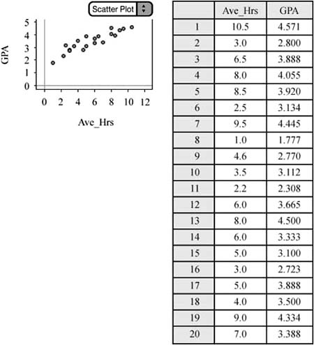
![]() Example 1: A group of teachers is interested in knowing whether a relationship exists between the average number of hours studied per week and high school cumulative grade point average (G.P.A.). The teachers obtain a random sample of students and determine the average number of hours each student studies along with the student’s cumulative high school G.P.A. Construct a 95% confidence interval for the true slope of the regression line to help answer the teachers’ question. Figure 10.1 presents a data table containing the average number of hours studied per week and the corresponding G.P.A for the 20 high-school students in the sample, along with a scatterplot of the data.
Example 1: A group of teachers is interested in knowing whether a relationship exists between the average number of hours studied per week and high school cumulative grade point average (G.P.A.). The teachers obtain a random sample of students and determine the average number of hours each student studies along with the student’s cumulative high school G.P.A. Construct a 95% confidence interval for the true slope of the regression line to help answer the teachers’ question. Figure 10.1 presents a data table containing the average number of hours studied per week and the corresponding G.P.A for the 20 high-school students in the sample, along with a scatterplot of the data.
Solution:
Step 1: We want to estimate β, the true slope of the regression line for the linear relationship between the average amount of time spent studying per week and the cumulative G.P.A. As always, we will check the assumptions and conditions necessary for inference.
Assumptions and conditions that verify:
Relationship has a linear form. The scatterplot in Figure 10.1 appears to be roughly linear.
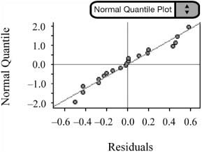
Residuals are independent. The residual plot in Figure 10.2 shows no obvious pattern.
Variability of residuals is constant. The residual plot in Figure 10.2 appears to have even spread.
Residuals are approximately normal. The normal probability plot (Figure 10.3) is approximately linear.

Step 2: With the assumptions and conditions for regression inference met, we are safe to construct a 95% confidence interval for the slope of the true regression line.

Step 3: We are 95% confident that the slope of the true regression line is between 0.1975 and 0.3151.
![]() Note that 0 is not included in the confidence interval. This implies that the slope of the regression line is not equal to zero. This means that there does appear to be a relationship between the average amount of time spent studying per week and a student’s cumulative grade point average.
Note that 0 is not included in the confidence interval. This implies that the slope of the regression line is not equal to zero. This means that there does appear to be a relationship between the average amount of time spent studying per week and a student’s cumulative grade point average.
![]() In order to find SEb and s, run the linear regression t-test on your graphing calculator, which gives s. You can then find
In order to find SEb and s, run the linear regression t-test on your graphing calculator, which gives s. You can then find ![]() by defining a list to be
by defining a list to be ![]() . For example, you could define L3 = (L1 – 5.64)2 and then use the sum and square root functions on your calculator. Again, in most cases, SEb and s will be given as computer output, and you’ll just have to substitute them into the formula.
. For example, you could define L3 = (L1 – 5.64)2 and then use the sum and square root functions on your calculator. Again, in most cases, SEb and s will be given as computer output, and you’ll just have to substitute them into the formula.
![]() We are now ready to discuss hypothesis testing for the slope β. If there is a relationship between the two quantitative variables of interest, the slope of the regression equation should be significantly different from zero.
We are now ready to discuss hypothesis testing for the slope β. If there is a relationship between the two quantitative variables of interest, the slope of the regression equation should be significantly different from zero.
![]() The null and alternative hypotheses for such a test are as follows:
The null and alternative hypotheses for such a test are as follows:
H0 : β = 0
Ha : β ≠ 0 (or < 0 or > 0)
As usual, the alternative hypothesis can be one-sided or two-sided.
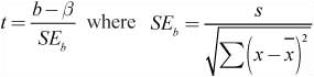
![]() The test-statistic associated with a test for the slope β is:
The test-statistic associated with a test for the slope β is:
![]() The assumptions and conditions for testing the slope β are the same as those for a confidence interval.
The assumptions and conditions for testing the slope β are the same as those for a confidence interval.
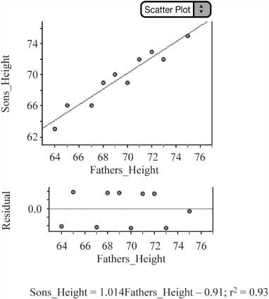
![]() Example 2: Is there reason to believe that a relationship exists between heights of fathers and the heights of their sons? To answer this question, use the following data in Figure 10.4, obtained from a random sample of 10 men and their sons. Test at the 5% level of significance.
Example 2: Is there reason to believe that a relationship exists between heights of fathers and the heights of their sons? To answer this question, use the following data in Figure 10.4, obtained from a random sample of 10 men and their sons. Test at the 5% level of significance.
| Father_Height | Sons_Height |
1 | 65 | 66 |
2 | 64 | 63 |
3 | 68 | 69 |
4 | 73 | 72 |
5 | 72 | 73 |
6 | 67 | 66 |
7 | 71 | 72 |
8 | 75 | 75 |
9 | 70 | 69 |
10 | 69 | 70 |
Figure 10.4. Heights of 10 randomly selected men and their sons.
Solution:
Step 1: We want to test the claim that there is a relationship between the heights of fathers and their sons. Let β = true slope of the least-squares regression line.
H0 : β = 0
Ha : β ≠ 0
Assumptions and conditions that verify:
Relationship has a linear form. The scatterplot in Figure 10.5 appears to be roughly linear.
Residuals are independent. The residual plot in Figure 10.6 shows no obvious pattern.
Variability of residuals is constant. The residual plot in Figure 10.6 appears to have even spread.
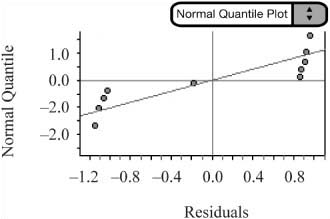
Residuals are approximately normal. The normal probability plot (Figure 10.7) is somewhat linear. Remember, if in doubt, you can always check a modified boxplot and look for skewness and outliers.

Step 2: With the assumptions and conditions for regression inference met, we are safe to proceed with the test for the true slope of the regression line.

Step 3: With a p-value of almost zero, we reject the null hypothesis at the 5% level. We conclude that the slope of the true regression line is different from zero and that there is a relationship between the heights of fathers and their sons.
![]() Note that the exact same procedures could be used to conduct a hypothesis test on rho, the correlation coefficient for the population.
Note that the exact same procedures could be used to conduct a hypothesis test on rho, the correlation coefficient for the population.
![]() Statistics for regression are often given in the form of a Minitab printout. You will come across these printouts as you do “released” exam questions in both the multiple-choice and free-response sections. Be sure to work through a few “released” exam questions that include these printouts. Your instructor will likely provide you with such printouts as well. Remember that there are almost always some “extra” statistics that you do not need. Don’t feel obligated to use all of the information from the printout. There may also be some statistics given that are not part of the AP Statistics curriculum. You can ignore what you don’t need. You’ll do great!
Statistics for regression are often given in the form of a Minitab printout. You will come across these printouts as you do “released” exam questions in both the multiple-choice and free-response sections. Be sure to work through a few “released” exam questions that include these printouts. Your instructor will likely provide you with such printouts as well. Remember that there are almost always some “extra” statistics that you do not need. Don’t feel obligated to use all of the information from the printout. There may also be some statistics given that are not part of the AP Statistics curriculum. You can ignore what you don’t need. You’ll do great!