6.1 Sampling Distributions
6.2 Sample Means and the Central Limit Theorem
6.3 Sample Proportions and the Central Limit Theorem
![]() Understanding sampling distributions is an integral part of inferential statistics. Recall that in inferential statistics you are making conclusions or assumptions about an entire population based on sample data. In this chapter, we will explore sampling distributions for means and proportions. In the remaining chapters, we will call upon the topics of this and previous chapters in order to study inferential statistics.
Understanding sampling distributions is an integral part of inferential statistics. Recall that in inferential statistics you are making conclusions or assumptions about an entire population based on sample data. In this chapter, we will explore sampling distributions for means and proportions. In the remaining chapters, we will call upon the topics of this and previous chapters in order to study inferential statistics.
![]() From this point on, it’s important that we understand the difference between a parameter and a statistic. A parameter is a number that describes some attribute of a population. For example, we might be interested in the mean, μ, and standard deviation, σ, of a population. There are many situations for which the mean and standard deviation of a population are unknown. In some cases, it is the population proportion that is not known. That is where inferential statistics comes in. We can use a statistic to estimate the parameter. A statistic is a number that describes an attribute of a sample. So, for the unknown μ we can use the sample mean,
From this point on, it’s important that we understand the difference between a parameter and a statistic. A parameter is a number that describes some attribute of a population. For example, we might be interested in the mean, μ, and standard deviation, σ, of a population. There are many situations for which the mean and standard deviation of a population are unknown. In some cases, it is the population proportion that is not known. That is where inferential statistics comes in. We can use a statistic to estimate the parameter. A statistic is a number that describes an attribute of a sample. So, for the unknown μ we can use the sample mean, ![]() , as an estimate of μ. It’s important to note that if we were to take another sample, we would probably get a different value for
, as an estimate of μ. It’s important to note that if we were to take another sample, we would probably get a different value for ![]() . In other words, if we keep sampling, we will probably keep getting different values for
. In other words, if we keep sampling, we will probably keep getting different values for ![]() (although some may be the same). Although μ may be unknown, it is a fixed number, as a population can have only one mean. The notation for the standard deviation of a sample is s. (Just remember that s is for “sample.”) We sometimes use s to estimate σ, as we will see in later chapters.
(although some may be the same). Although μ may be unknown, it is a fixed number, as a population can have only one mean. The notation for the standard deviation of a sample is s. (Just remember that s is for “sample.”) We sometimes use s to estimate σ, as we will see in later chapters.
![]() To summarize the notation, remember that the symbols μ and σ (parameters) are used to denote the mean and standard deviation of a population, and
To summarize the notation, remember that the symbols μ and σ (parameters) are used to denote the mean and standard deviation of a population, and ![]() and s (statistics) are used to denote the mean and standard deviation of a sample. You might find it helpful to remember that s stands for “statistic” and “sample” while p stands for “parameter” and “population.” You should also remember that Greek letters are typically used for population parameters. Be sure to use the correct notation! It can help convince the reader (grader) of your AP* Exam that you understand the difference between a sample and a population.
and s (statistics) are used to denote the mean and standard deviation of a sample. You might find it helpful to remember that s stands for “statistic” and “sample” while p stands for “parameter” and “population.” You should also remember that Greek letters are typically used for population parameters. Be sure to use the correct notation! It can help convince the reader (grader) of your AP* Exam that you understand the difference between a sample and a population.
![]() Consider again a population with an unknown mean, μ. Sometimes it is simply too difficult or costly to determine the true mean, μ. When this is the case, we then take a random sample from the population and find the mean of the sample,
Consider again a population with an unknown mean, μ. Sometimes it is simply too difficult or costly to determine the true mean, μ. When this is the case, we then take a random sample from the population and find the mean of the sample, ![]() . As mentioned earlier, we could repeat the sampling process many, many times. Each time we would recalculate the mean, and each time we might get a different value. This is called sampling variability. Remember, μ does not change. The population mean for a given population is a fixed value. The sample mean,
. As mentioned earlier, we could repeat the sampling process many, many times. Each time we would recalculate the mean, and each time we might get a different value. This is called sampling variability. Remember, μ does not change. The population mean for a given population is a fixed value. The sample mean, ![]() , on the other hand, changes depending on which individuals from the population are chosen. Sometimes the value of
, on the other hand, changes depending on which individuals from the population are chosen. Sometimes the value of ![]() will be greater than the true population mean, μ, and other times
will be greater than the true population mean, μ, and other times ![]() will be smaller than μ. This means that
will be smaller than μ. This means that ![]() is an unbiased estimator of μ.
is an unbiased estimator of μ.
![]() The sampling distribution is the distribution of the values of the statistic if all possible samples of a given size are taken from the population. Don’t confuse samples with sampling distributions. When we talk about sampling distributions, we are not talking about one sample; we are talking about all possible samples of a particular size that we could obtain from a given population.
The sampling distribution is the distribution of the values of the statistic if all possible samples of a given size are taken from the population. Don’t confuse samples with sampling distributions. When we talk about sampling distributions, we are not talking about one sample; we are talking about all possible samples of a particular size that we could obtain from a given population.
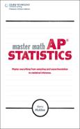
![]() Example 1: Consider the experiment of rolling a pair of standard six-sided dice. There are 36 possible outcomes. If we define μ to be the average of the two dice, we can look at all 36 values in the sampling distribution of
Example 1: Consider the experiment of rolling a pair of standard six-sided dice. There are 36 possible outcomes. If we define μ to be the average of the two dice, we can look at all 36 values in the sampling distribution of ![]() (Figure 6.1). If we averaged all 36 possible values of
(Figure 6.1). If we averaged all 36 possible values of ![]() , we would obtain the exact value of μ x. This is always the case.
, we would obtain the exact value of μ x. This is always the case.
![]() As mentioned, sometimes the value of
As mentioned, sometimes the value of ![]() is below μ, and sometimes it is above μ. In Example 1, you can see that the center of the sampling distribution is exactly 3.5. In other words, the statistic,
is below μ, and sometimes it is above μ. In Example 1, you can see that the center of the sampling distribution is exactly 3.5. In other words, the statistic, ![]() , is unbiased because the mean of the sampling distribution is equal to the true value of the parameter being tested, which is μ. Although the values of
, is unbiased because the mean of the sampling distribution is equal to the true value of the parameter being tested, which is μ. Although the values of ![]() may differ, they do not tend to consistently overestimate or underestimate the true mean of the population.
may differ, they do not tend to consistently overestimate or underestimate the true mean of the population.
![]() As you will see later in this chapter, larger samples have less variability when it comes to sampling distributions. The spread is determined by how the sample is designed as well as the size of the sample. It’s also important to note that the variability of the sampling distribution for a particular sample size does not depend on the size of the population from which the sample is obtained. An SRS (simple random sample) of size 4000 from the population of U.S. residents has approximately the same variability as an SRS of size 4000 from the population of Indiana residents. However, in order for the variability to be the same, both samples must be the same size and be obtained in the same manner. We want our samples to be obtained from correct sampling methods and the sample size to be large enough that our samples have low bias and low variability.
As you will see later in this chapter, larger samples have less variability when it comes to sampling distributions. The spread is determined by how the sample is designed as well as the size of the sample. It’s also important to note that the variability of the sampling distribution for a particular sample size does not depend on the size of the population from which the sample is obtained. An SRS (simple random sample) of size 4000 from the population of U.S. residents has approximately the same variability as an SRS of size 4000 from the population of Indiana residents. However, in order for the variability to be the same, both samples must be the same size and be obtained in the same manner. We want our samples to be obtained from correct sampling methods and the sample size to be large enough that our samples have low bias and low variability.
![]() The following activity will help you understand the difference between a population and a sample, sampling distributions, sampling variability, and the Central Limit Theorem. I learned of this activity a few years ago from AP Statistics consultant and teacher Chris True. I am not sure where this activity originated, but it will help you understand the concepts presented in this chapter. If you’ve done this activity in class, that’s great! Read through the next few pages anyway, as it will provide you with a good review of sampling and the Central Limit Theorem.
The following activity will help you understand the difference between a population and a sample, sampling distributions, sampling variability, and the Central Limit Theorem. I learned of this activity a few years ago from AP Statistics consultant and teacher Chris True. I am not sure where this activity originated, but it will help you understand the concepts presented in this chapter. If you’ve done this activity in class, that’s great! Read through the next few pages anyway, as it will provide you with a good review of sampling and the Central Limit Theorem.
![]() The activity begins with students collecting pennies that are currently in circulation. Students bring in enough pennies over the period of a few days such that I get a total of about 600 to 700 pennies between all of my AP Statistics classes. Students enter the dates of the pennies into the graphing calculator (and Fathom) as they place the pennies into a container. These 600 to 700 pennies become our population of pennies. Then students make a guess as to what they think the distribution of our population of pennies will look like. Many are quick to think that the distribution of the population of pennies is approximately normal. After some thought and discussion about the dates of the pennies in the population, students begin to understand that the population distribution is not approximately normal but skewed to the left. Once we have discussed what we think the population distribution should look like, we examine a histogram or dotplot of the population of penny dates. As you can see in Figure 6.2, the distribution is indeed skewed to the left.
The activity begins with students collecting pennies that are currently in circulation. Students bring in enough pennies over the period of a few days such that I get a total of about 600 to 700 pennies between all of my AP Statistics classes. Students enter the dates of the pennies into the graphing calculator (and Fathom) as they place the pennies into a container. These 600 to 700 pennies become our population of pennies. Then students make a guess as to what they think the distribution of our population of pennies will look like. Many are quick to think that the distribution of the population of pennies is approximately normal. After some thought and discussion about the dates of the pennies in the population, students begin to understand that the population distribution is not approximately normal but skewed to the left. Once we have discussed what we think the population distribution should look like, we examine a histogram or dotplot of the population of penny dates. As you can see in Figure 6.2, the distribution is indeed skewed to the left.

![]() It’s important to discuss the shape, center, and spread of the distribution. As just stated, the shape of the distribution of the population of pennies is skewed left. The mean, which we will use as a measure of center, is μ = 1990.5868. Since we are using the mean as the measure of center, it makes sense to use the standard deviation to measure spread. For this population of 651 pennies, σ = 12.6937 years.
It’s important to discuss the shape, center, and spread of the distribution. As just stated, the shape of the distribution of the population of pennies is skewed left. The mean, which we will use as a measure of center, is μ = 1990.5868. Since we are using the mean as the measure of center, it makes sense to use the standard deviation to measure spread. For this population of 651 pennies, σ = 12.6937 years.
![]() Once we’ve discussed the shape, center, and spread of the population distribution, we begin sampling. Students work in pairs and draw out several samples of each of the sizes: 4, 9, 16, 25, and 50. Sampling variability becomes apparent as students repeat samples for the various sample sizes. We divide up the sampling task among the students in class so that when we are done we have about 100 to 120 samples for each sample size. We graph the sampling distribution for each sample size and compute the mean and standard deviation of each sampling distribution.
Once we’ve discussed the shape, center, and spread of the population distribution, we begin sampling. Students work in pairs and draw out several samples of each of the sizes: 4, 9, 16, 25, and 50. Sampling variability becomes apparent as students repeat samples for the various sample sizes. We divide up the sampling task among the students in class so that when we are done we have about 100 to 120 samples for each sample size. We graph the sampling distribution for each sample size and compute the mean and standard deviation of each sampling distribution.
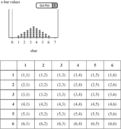
![]() We can then analyze the sampling distribution for each sample size. We begin with n = 4 (Figure 6.3).
We can then analyze the sampling distribution for each sample size. We begin with n = 4 (Figure 6.3).
![]() Again, think about the shape, center, and spread of the distribution. Remember, this is a sampling distribution. This is the distribution of about 100 samples of size 4. As you can see in Figure 6.3, the shape of the sampling distribution is different from that of the population. Although the shape of the population is skewed left, the shape of the sampling distribution for n = 4 is more symmetrical. The center of the sampling distribution is μ
Again, think about the shape, center, and spread of the distribution. Remember, this is a sampling distribution. This is the distribution of about 100 samples of size 4. As you can see in Figure 6.3, the shape of the sampling distribution is different from that of the population. Although the shape of the population is skewed left, the shape of the sampling distribution for n = 4 is more symmetrical. The center of the sampling distribution is μ![]() = 1990.6636, which is very close to the population mean, μ. The spread of the sampling distribution is σ
= 1990.6636, which is very close to the population mean, μ. The spread of the sampling distribution is σ![]() = 6.6031. We can visualize that the spread of the sampling distribution is less than that of the population and that the mean of the sampling distribution (balancing point) is around 1990 to 1991. Note that if we had obtained all samples of size 4 from the population, then
= 6.6031. We can visualize that the spread of the sampling distribution is less than that of the population and that the mean of the sampling distribution (balancing point) is around 1990 to 1991. Note that if we had obtained all samples of size 4 from the population, then
Although it’s impractical to obtain all possible samples of size 4 from the population of 651 pennies, our results are very close to what we would obtain if we had obtained all 7,414,857,450 samples. That's right; from a population of 651 pennies, the number of samples of size 4 you could obtain is

![]() The following sampling distribution is for samples of size n = 9 (Figure 6.4).
The following sampling distribution is for samples of size n = 9 (Figure 6.4).

![]() The sampling distribution for samples of size n = 9 is more symmetrical than the sampling distribution for n = 4. The mean and standard deviation for this sampling distribution are μ
The sampling distribution for samples of size n = 9 is more symmetrical than the sampling distribution for n = 4. The mean and standard deviation for this sampling distribution are μ![]() ≈ 1990.1339 and σ
≈ 1990.1339 and σ![]() ≈ 4.8852. Again, we can visualize that the mean is around 1990 to 1991 and that the spread is less for this distribution than that for n = 4.
≈ 4.8852. Again, we can visualize that the mean is around 1990 to 1991 and that the spread is less for this distribution than that for n = 4.
![]() The following sampling distribution is for samples of size n = 16 (Figure 6.5).
The following sampling distribution is for samples of size n = 16 (Figure 6.5).

![]() The sampling distribution for samples of size n = 16 is more symmetrical than the sampling distribution for n = 9. The mean and standard deviation for this sampling distribution are μ
The sampling distribution for samples of size n = 16 is more symmetrical than the sampling distribution for n = 9. The mean and standard deviation for this sampling distribution are μ![]() ≈ 1990.4912 and σ
≈ 1990.4912 and σ![]() ≈ 4.3807. Again, we can visualize that the mean is around 1990 to 1991 and that the spread is less for this distribution than that for n = 9.
≈ 4.3807. Again, we can visualize that the mean is around 1990 to 1991 and that the spread is less for this distribution than that for n = 9.
![]() Notice the outlier of 1968. Although it’s possible to obtain a sample of size n = 16 with a sample average of 1968 from our population of pennies, it is very unlikely. This is probably a mistake on the part of the student reporting the sample average or on the part of the student recording the sample average. It’s interesting to note the impact that the outlier has on the variability of the sampling distribution. The theoretical standard deviation for the sampling distribution is
Notice the outlier of 1968. Although it’s possible to obtain a sample of size n = 16 with a sample average of 1968 from our population of pennies, it is very unlikely. This is probably a mistake on the part of the student reporting the sample average or on the part of the student recording the sample average. It’s interesting to note the impact that the outlier has on the variability of the sampling distribution. The theoretical standard deviation for the sampling distribution is
Notice that the standard deviation of our sampling distribution is greater than this value, which is due largely to the outlier of 1968. This provides us with a good reminder that the mean and standard deviation are not resistant measures. That is to say that they can be greatly influenced by extreme observations.
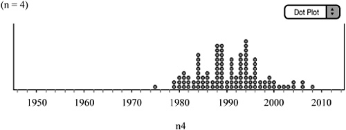
![]() The following is the sampling distribution obtained for n = 25 (Figure 6.6).
The following is the sampling distribution obtained for n = 25 (Figure 6.6).
![]() The mean and standard deviation for this sampling distribution are μ
The mean and standard deviation for this sampling distribution are μ![]() ≈ 1990.75 and σ
≈ 1990.75 and σ![]() ≈ 2.5103. The shape of the sampling distribution is more symmetrical and more normal. We can visualize that the center of the distribution is again around 1990 to 1991 and that the variability is continuing to decrease as the sample size gets larger.
≈ 2.5103. The shape of the sampling distribution is more symmetrical and more normal. We can visualize that the center of the distribution is again around 1990 to 1991 and that the variability is continuing to decrease as the sample size gets larger.
![]() The following is the sampling distribution obtained for n = 50 (Figure 6.7).
The following is the sampling distribution obtained for n = 50 (Figure 6.7).
![]() The mean and standard deviation for this sampling distribution are μ
The mean and standard deviation for this sampling distribution are μ![]() ≈ 1990.4434 and σ
≈ 1990.4434 and σ![]() ≈ 3.0397. The shape of the sampling distribution is more normal than that of any of the sampling distributions of smaller sample sizes. The center can again be visualized to be around 1990 to 1991, and the spread can be visualized to be smaller that that of the sampling distributions of smaller sample sizes. Notice, however, that the standard deviation of the sampling distribution is actually larger than that of size n = 25. How can this happen? Notice that there are two outliers. My students called them “super outliers.” These are responsible for making the standard deviation of the sampling distribution larger than it would be theoretically. These outliers are very, very unlikely. We would be more likely to be struck by lightning twice while winning the lottery than to obtain two outliers as extreme as these. The outliers are probably due to human error in recording or calculating the sample means.
≈ 3.0397. The shape of the sampling distribution is more normal than that of any of the sampling distributions of smaller sample sizes. The center can again be visualized to be around 1990 to 1991, and the spread can be visualized to be smaller that that of the sampling distributions of smaller sample sizes. Notice, however, that the standard deviation of the sampling distribution is actually larger than that of size n = 25. How can this happen? Notice that there are two outliers. My students called them “super outliers.” These are responsible for making the standard deviation of the sampling distribution larger than it would be theoretically. These outliers are very, very unlikely. We would be more likely to be struck by lightning twice while winning the lottery than to obtain two outliers as extreme as these. The outliers are probably due to human error in recording or calculating the sample means.
![]() The penny activity is the Central Limit Theorem (the Fundamental Theorem of Statistics) at work. The Central Limit Theorem says that as the sample size increases, the mean of the sampling distribution of
The penny activity is the Central Limit Theorem (the Fundamental Theorem of Statistics) at work. The Central Limit Theorem says that as the sample size increases, the mean of the sampling distribution of ![]() approaches a normal distribution with mean μ and standard deviation,
approaches a normal distribution with mean μ and standard deviation,
This is true for any population, not just normal populations! How large the sample must be depends on the shape of the population. The more non-normal the population, the larger the sample size needs to be in order for the sampling distribution to be approximately normal. Most textbooks consider 30 or 40 to be a “large” sample. The Central Limit Theorem allows us to use normal calculations when we are dealing with non-normal populations, provided that the sample size is large. It is important to remember that μ![]() ≈ μ and
≈ μ and ![]() for any sampling distribution of the mean. The Central Limit Theorem states that the shape of the sampling distribution becomes more normal as the sample size increases.
for any sampling distribution of the mean. The Central Limit Theorem states that the shape of the sampling distribution becomes more normal as the sample size increases.
![]() Now that we’ve discussed sampling distributions, sample means, and the Central Limit Theorem, it’s time to turn our attention to sample proportions. Before we begin our discussion, it’s important to note that when referring to a sample proportion, we always use
Now that we’ve discussed sampling distributions, sample means, and the Central Limit Theorem, it’s time to turn our attention to sample proportions. Before we begin our discussion, it’s important to note that when referring to a sample proportion, we always use ![]() . When referring to a population proportion, we always use p. Note that some texts use π instead of p. In this case, π is just a Greek letter being used to denote the population proportion, not 3.1415 …
. When referring to a population proportion, we always use p. Note that some texts use π instead of p. In this case, π is just a Greek letter being used to denote the population proportion, not 3.1415 …
![]() The Central Limit Theorem also applies to proportions as long as the following conditions apply:
The Central Limit Theorem also applies to proportions as long as the following conditions apply:
The sampled values must be independent of one another. Sometimes this is referred to as the 10% condition. That is, the sample size must be only 10% of the population size or less. If the sample size is larger than 10% of the population, it is unlikely that the individuals in the sample would be independent.
The sample must be large enough. A general rule of thumb is that np ≥ 10 and n(1 − p) ≥ 10. As always, the sample must be random.
![]() If these two conditions are met, the sampling distribution of
If these two conditions are met, the sampling distribution of ![]() should be approximately normal. The mean of the sampling distribution of
should be approximately normal. The mean of the sampling distribution of ![]() is exactly equal to p. The standard deviation of the sampling distribution is equal to:
is exactly equal to p. The standard deviation of the sampling distribution is equal to:

![]() Note that because the average of all possible
Note that because the average of all possible ![]() values is equal to p, the sample proportion,
values is equal to p, the sample proportion, ![]() , is an unbiased estimator of the population proportion, p.
, is an unbiased estimator of the population proportion, p.
![]() Also notice how the sample size affects the standard deviation. Notice that as n gets larger, the fraction
Also notice how the sample size affects the standard deviation. Notice that as n gets larger, the fraction ![]() gets smaller. Thus, as the sample size increases, the variability in the sampling distribution decreases. This is the same concept discussed in the penny activity. Note also that for any sample size n, the standard deviation is largest from a population with p = 0.50.
gets smaller. Thus, as the sample size increases, the variability in the sampling distribution decreases. This is the same concept discussed in the penny activity. Note also that for any sample size n, the standard deviation is largest from a population with p = 0.50.