An understanding of the concept of randomness is essential for tackling the concept of probability. What does it mean for something to be random? AP Statistics students usually have a fairly good concept of what it means for something to be random and have likely done some probability calculations in their previous math courses. I’m always a little surprised, however, when we use the random integer function of the graphing calculator when randomly assigning students to their seats or assigning students to do homework problems on the board. It’s almost as if students expect everyone in the class to be chosen before they are chosen for the second or third time. Occasionally, a student’s number will come up two or even three times before someone else’s, and students will comment that the random integer function on the calculator is not random. Granted, it’s unlikely for this to happen with 28 students in the class, but not impossible. Think about rolling a standard six-sided die. The outcomes associated with this event are random—that is, they are uncertain but follow a predictable distribution over the long run. The proportion associated with rolling any one of the six sides of the die over the long run is the probability of that outcome.

It’s important to understand what is meant by in the long run. When I assign students to their seats or use the random integer function of the graphing calculator to assign students to put problems on the board, we are experiencing what is happening in the short run. The Law of Large Numbers tells us that the long-run relative frequency of repeated, independent trials gets closer to the expected relative frequency once the number of trials increases. Events that seem unpredictable in the short run will eventually “settle down” after enough trials are accumulated. This may require many, many trials. The number of trials that it takes depends on the variability of the random variable of interest. The more variability, the more trials it takes. Casinos and insurance companies use the Law of Large Numbers on an everyday basis. Averaging our results over many, many individuals produces predictable results. Casinos are guaranteed to make a profit because they are in it for the long run whereas the gambler is in it for the relative short run.

The probability of an event is always a number between 0 and 1, inclusive. Sometimes we consider the theoretical probability and other times we consider the empirical probability. Consider the experiment of flipping a fair coin. The theoretical probability of the coin landing on either heads or tails is equal to 0.5. If we actually flip the coin a 100 times and it lands on tails 40 times, then the empirical probability is equal to 0.4. If the empirical probability is drastically different from the theoretical probability, we might consider whether the coin is really fair. Again, we would want to perform many, many trials before we conclude that the coin is unfair.

Example 1: Consider the experiment of flipping a fair coin three times. Each flip of the coin is considered a trial and each trial for this experiment has two possible outcomes, heads or tails. A list containing all possible outcomes of the experiment is called a sample space. An event is a subset of a sample space. A tree diagram can be used to organize the outcomes of the experiment, as shown in Figure 5.1.

Figure 5.1. Tree diagram.

Tree diagrams can be useful in some problems that deal with probability. Each trial consists of one line in the tree diagram, and each branch of the tree diagram can be labeled with the appropriate probability. Working our way down and across the tree diagram, we can obtain the eight possible outcomes in the sample space. S = {HHH, HHT, HTH, HTT, THH, THT, TTH, TTT} To ensure that we have the correct number of outcomes listed in the sample space, we could use the counting principle, or multiplication principle. The multiplication principle states that if you can do task 1 in m ways and you can do task 2 in n ways, then you can do task 1 followed by task 2 in m × n ways. In this experiment we have three trials, each with two possible outcomes. Thus, we would have 2 × 2 × 2 = 8 possible outcomes in the sample space.

Example 2: Let’s continue with the experiment discussed in Example 1. What’s the probability of flipping the coin three times and obtaining heads all three times?

Solution: We can answer that question in one of two ways. First, we could use the sample space. HHH is one of eight possible (equally likely) outcomes listed in the sample space, so P(HHH) = ⅛. The second method we could use to obtain P(HHH) is to use the concept of independent events. Two events are independent if the occurrence or non-occurrence of one event does not alter the probability of the second event. The trials of flipping a coin are independent. Whether or not the first flip results in heads or tails does not change the probability of the coin landing on heads or tails for the second or third flip. If two events are independent, then P(A ∩ B) = P(A and B) = P(A) • P(B). We can apply this concept to this experiment. P(HHH) = (½) • (½) • (½) = ⅛. Later on, in Example 11, we will show how to prove whether or not two events are independent.

Example 3: Again consider Example 1. Find the probability of obtaining at least one tail (not all heads).

Solution: The events “all heads” and “at least one tail” are complements. The set “at least one tail” is the set of all outcomes from the sample space excluding “all heads.” All the outcomes in a given sample space should sum to one, and so any two events that are complements should sum to one as well. Thus, the probability of obtaining “at least one tail” is equal to: 1 − P(HHH) = 1 − ⅛ = ⅞. We can verify our answer by examining the sample space we obtained in Example 1 and noting that 7 out of the 8 equally likely events in the sample space contain at least one tail. Typical symbols for the complement of event A are: A^c, A′, or Ā.

Example 4: Consider the experiment of drawing two cards from a standard deck of 52 playing cards. Find the probability of drawing two hearts if the first card is replaced and the deck is shuffled before the second card is drawn. The following tree diagram can be used to help answer the question.

Figure 5.2. Tree diagram with replacement.

Solution: Let H = “heart” and Hc = “ non – heart” Notice that the probability of the second card being a heart is independent of the first card being a heart. Thus, P(HH) = ¼ • ¼ = 1/16.

Example 5: How would Example 4 change if the first card were not replaced before the second card was drawn? Find the probability of drawing two hearts if the first card drawn is not replaced before the second card is drawn. Notice how the probabilities in the tree diagram change depending on whether or not a heart is drawn as the first card.

Figure 5.3. Tree diagram without replacement.

When two events A and B are not independent, then P(A ∩ B) = P(A) • P(B | A) This is a conditional probability, which we will discuss in more detail in section 5.2. Applying this formula, we obtain P(HHH) = 13/52 • 12/51 = 1/17.

Example 6: Suppose that in a particular high school the probability that a student takes AP Statistics is equal to 0.30 (call this event A), and the probability that a student takes AP Calculus is equal to 0.45 (call this event B.) Suppose also that the probability that a student takes both AP Statistics and AP Calculus is equal to 0.10. Find the probability that a student takes either AP Statistics or AP Calculus.

Solution: We can organize the information given in a Venn diagram as shown in Figure 5.4.

Figure 5.4. Venn diagram for two events, A and B.

Notice the probability for each section of the Venn diagram. The total circle for event A (AP Statistics) has probabilities that sum to 0.30 and the total circle for event B (AP Calculus) has probabilities that sum to 0.45. Also notice that all four probabilities in the Venn diagram sum to 1. We can use the General Addition Rule for the Union of Two Events. P(A ∪ B) = P(A) + P(B) − P(B) − P(A ∩ B) Note that ∪ (union) means “or” and ∩ (intersection) means “and.” We could then apply the formula as follows:

If you consider the Venn diagram, the General Addition Rule makes sense. When you consider event A, you are adding in the “overlapping” of the two circles (student takes AP Stats and AP Calculus), and when you consider event B, you are again adding in the “overlapping” of the two circles. Thus, the General Addition Rule has us subtracting the intersection of the two circles, which is the “overlapping” section.

Example 7: Reconsider Example 6. Find the probability that a student takes neither AP Statistics nor AP Calculus.

Solution: From the Venn diagram in Figure 5.4 we can see that the probability that a student takes neither course is the area (probability) on the outside of the circles, which is 0.35. We could also conclude that 20% of students take AP Statistics but not AP Calculus and that 35% of students take AP Calculus but not AP Statistics.

Example 8: Referring again to Example 6, suppose that AP Statistics and AP Calculus are taught only once per day and during the same period. It would then be impossible for a student to take both AP Statistics and AP Calculus. How would the Venn diagram change?

Solution: We could construct the Venn diagram as shown in Figure 5.5.

Figure 5.5. Venn diagram for disjoint (mutually exclusive) events.

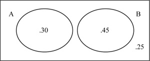
Notice that the circles are not overlapping since events A and B cannot occur at the same time. Events A and B are disjoint, or mutually exclusive. This implies that P(A ∩ B) = 0. Applying the General Addition Rule, we obtain: P(A ∪ B) = 0.30 + 0.45 = 0.75. Notice that we do not have to subtract P(A ∩ B) since it is equal to 0. Thus, for disjoint events:

Don’t confuse independent events and disjoint (mutually exclusive) events. Try to keep these concepts separate, but remember that if you know two events are independent, they cannot be disjoint. The reverse is also true. If two events are disjoint, then they cannot be independent. Think about Example 8, where it was impossible to take AP Statistics and AP Calculus at the same time (disjoint events.) If a student takes AP Statistics, then the probability that they take AP Calculus changes from 0.35 to zero. Thus, these two events, which are disjoint, are not independent. That is, taking AP Statistics changes the probability of taking AP Calculus. It’s also worth noting that some events are neither disjoint nor independent. The fact that an event is not independent does not necessarily mean it’s disjoint and vice versa. Consider drawing two cards at random, without replacement, from a standard deck of 52 playing cards. The events “first card is an ace” and “second card is an ace” are neither disjoint nor independent. The events are not independent because the probability of the second card being an ace depends on whether or not an ace was drawn as the first card. The events are not disjoint because it is possible that the first card is an ace and the second card is also an ace.

Example 9: Example 5 is a good example of what we mean by conditional probability. That is, finding a given probability if it is known that another event or condition has occurred or not occurred. Knowing whether or not a heart was chosen as the first card determines the probability that the second card is a heart. We can find P(2nd card heart / 1st card heart) by using the formula given in Example 5 and solving for P(A | B), read A given B.

Thus,

When applying the formula, just remember that the numerator is always the intersection (“and”) of the events, and the denominator is always the event that comes after the “given that” line. Applying the formula, we obtain:

The formula works, although we could have just looked at the tree diagram and avoided using the formula. Sometimes we can determine a conditional probability simply by using a tree diagram or looking at the data, if it’s given. The next problem is a good example of a problem where the formula for conditional probability really comes in handy.

Example 10: Suppose that a medical test can be used to determine if a patient has a particular disease. Many medical tests are not 100% accurate. Suppose the test gives a positive result 90% of the time if the person really has the disease and also gives a positive result 1% of the time when a person does not have the disease. Suppose that 2% of a given population actually have the disease. Find the probability that a randomly chosen person from this population tests positive for the disease.

Solution: We can use a tree diagram to help us solve the problem (Figure 5.6).

Figure 5.6. Tree diagram for conditional probability.

It’s important to note that the test can be positive whether or not the person actually has the disease. We must consider both cases. Let event D = Person has the disease and let event D^c = Person does not have the disease. Let ″pos″ = positive and ″neg″ = negative.

Thus, the probability that a randomly chosen person tests positive for the disease is 0.0278.

Example 11: Referring to Example 10, find the probability that a randomly chosen person has the disease given that the person tested positive. In this case we know that the person tested positive and we are trying to find the probability that they actually have the disease. This is a conditional probability known as Bayes’s Rule.

You should understand that Bayes’s Rule is really just an extended conditional probability rule. However, it’s probably unnecessary for you to remember the formula for Bayes’s Rule. If you understand how to apply the conditional probability formula and you can set up a tree diagram, you should be able to solve problems involving Bayes’s Rule. Just remember that to find P(pos) you have to consider that a positive test result can occur if the person has the disease and if the person does not have the disease.

Again, in some problems you may be given the probabilities and need to use the conditional probability formula and in others it may be unnecessary. In the following example, the formula for conditional probability certainly works, but using it is unnecessary. All the data needed to answer the conditional probability is given in the table (Figure 5.7).

Example 12: Consider a marathon in which 38,500 runners participate. Figure 5.7 contains the times of the runners broken down by age. Find the probability that a randomly chosen runner runs under 3 hours given that they are in the 50+ age group.

Solution: Although we could use the conditional probability formula, it’s really unnecessary. It’s given that the person chosen is in the 50+ age group, which means instead of dividing by the total number of runners (38,500) we can simply divide the number of runners that are both 50+ and ran under 3 hours by the total number of 50+ runners.

Thus, the probability that a randomly chosen person runs under 3 hours for the marathon given that they are 50 or older is about 0.0031.

Example 13: Let’s revisit independent events. Is the age of a runner independent of the time that the runner finishes the marathon? It doesn’t seem likely that the two events are independent of one another. We would expect older runners to run slower, on average, than younger runners. There are certainly exceptions to this rule, which I am reminded of when someone ten years older than me finishes before me in a marathon! Are the events “finishes under 3 hours” and “50+ age group” independent of one another?

Solution: Remember, if the two events are independent then:

Thus, P(under 3 hrs and 50+) = P(under 3 hrs) • P(50+)

We can again use the table values from Figure 5.7 to answer this question.

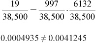
Since the two are not equal, the events are not independent.

Now that we’ve discussed the concepts of randomness and probability, we turn our attention to random variables. A random variable is a numeric variable from a random experiment that can take on different values. The random variable can be discrete or continuous. A discrete random variable, X, is a random variable that can take on only a countable number. (In some cases a discrete random variable can take on a finite number of values and in others it can take on an infinite number of values.) For example, if I roll a standard six-sided die, there are only six possible values of X, which can take on the values 1, 2, 3, 4, 5, or 6. I can then create a valid probability distribution for X, which lists the values of X and the corresponding probability that X will occur (Figure 5.8).

The probabilities in a valid probability distribution must all be between 0 and 1 and all probabilities must sum to 1.

Example 14: Consider the experiment of rolling a standard (fair) six-sided die and the probability distribution in Figure 5.8. Find the probability of rolling an odd number greater than 1.

Solution: Remember that this is a discrete random variable. This means that rolling an odd number greater than 1 is really rolling a 3 or a 5. Also note that we can’t roll a 3 and a 5 with one roll of the die, which makes the events disjoint or mutually exclusive. We can simply add the probabilities of rolling a 3 and a 5.

We sometimes need to find the mean and variance of a discrete random variable. We can accomplish this by using the following formulas:

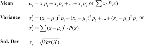
Recall that the standard deviation is the square root of the variance, so once we’ve found the variance it is easy to find the standard deviation. It’s important to understand how the formulas work. Remember that the mean is the center of the distribution. The mean is calculated by summing up the product of all values that the variable can take on and their respective probabilities. The more likely a given value of X, the more that value of X is “weighted” when we calculate the mean. The variance is calculated by averaging the squared deviations for each value of X from the mean.

Example 15: Again consider rolling a standard six-sided die and the probability distribution in Figure 5.8. Find the mean, variance, and standard deviation for this experiment.

Solution: We can apply the formulas for the mean and variance as follows:

Notice that since the six sides of the die are equally likely, it seems logical that the mean of this discrete random variable is equal to 3.5. As always, it’s important to show your work when applying the appropriate formulas. Note that you can also utilize the graphing calculator to find the mean, variance, and standard deviation of a discrete random variable. But be careful! Some calculators give the standard deviation, not the variance. That’s not a problem, however; if you know the standard deviation, you can simply square it to get the variance. You can find the standard deviation of a discrete random variable on the TI83/84 graphing calculator by creating list one to be the values that the discrete random variable takes on and list two to be their respective probabilities. You can then use the one-variable stats option on your calculator to find the standard deviation. Caution! You must specify that you want one-variable stats for list one and list two (1-Var Stats L₁,L₂). Otherwise your calculator will only perform one-variable stats on list one.

Example 16: Suppose a six-sided die with sides numbered 1–6 is loaded in such a way that in the long run you would expect to have twice as many “1’s” and twice as many “2’s” as any other outcome. Find the probability distribution for this experiment, and then find the mean and standard deviation.

Solution: See Figure 5.9.

Since we are dealing with a valid probability distribution, we know that all probabilities must sum to 1.

We can then complete the probability distribution as follows (Figure 5.10).

We can then find the mean and standard deviation by applying the formulas and using our calculators.

Notice that the mean is no longer 3.5. The loaded die “weights” two sides of the die so that they occur more frequently, which lowers the mean from 3.5 on the standard die to 3 on the loaded die.

Some random variables are not discrete—that is, they do not always take on values that are countable numbers. The amount of time that it takes to type a five-page paper, the time it takes to run the 100 meter dash, and the amount of liquid that can travel through a drainage pipe are all examples of continuous random variables.

A continuous random variable is a random variable that can take on values that comprise an interval of real numbers. When dealing with probability distributions for continuous random variables we often use density curves to model the distributions. Remember that any density curve has area under the curve equal to one. The probability for a given event is the area under the curve for the range of values of X that make up the event. Since the probability for a continuous random variable is modeled by the area under the curve, the probability of X being one specific value is equal to zero. The event being modeled must be for a range of values, not just one value of X. Think about it this way: The area for one specific value of X would be a line and a line has area equal to zero. This is an important distinction between discrete and continuous random variables. Finding P(X ≥ 3) and P(X > 3) would produce the same result if we were dealing with a continuous random variable since P(X = 3) = 0.Finding P(X ≥ 3) and P(X > 3) would probably produce different results if we were dealing with a discrete random variable. In this case, X > 3 would begin with 4 because 4 is the first countable number greater than 3. X ≥ 3 would include 3.

It is sometimes necessary to perform basic operations on random variables. Suppose that X is a random variable of interest. The expected value (mean) of X would be μ_x and the variance would be σ_x². Suppose also that a new random variable Z can be defined such that Z = a ± bx. The mean and variance of Z can be found by applying the following Rules for Means and Variances:

Example 17: Given a random variable X with μ_x = 4 and σ_x = 1.2, find μ_z, σ_z² and σ_z given that Z = 3 + 4X.

Solution: Instead of going back to all values of X and multiplying all values by 4 and adding 3, we can simply use the mean, variance, and standard deviation of X and apply the Rules for Means and Variances.

Think about it. If all values of X were multiplied by 4 and added to 3, the mean would change in the same fashion. We can simply take the mean of X, multiply it by 4, and then add 3.

The variability (around the mean) would be increased by multiplying the values of X by 4. However, adding 3 to all the values of X would increase the values of X by 3 but would not change the variability of the values around the new mean. Adding 3 does not change the variability, so the Rules for Variances does not have us add 3, but rather just multiply by 4 or 4² depending on whether we are working with the standard deviation or variance. If we are finding the new standard deviation, we multiply by 4; if we are finding the new variance, we multiply by 4² or 16. When dealing with the variance we multiply by the factor squared. This is due to the relationship between the standard deviation and variance. Remember that the variance is the square of the standard deviation.

Notice that 4.8² = 23.04.

Sometimes we wish to find the sum or difference of two random variables. If X and Y are random variables, we can use the following to find the mean of the sum or difference:

We can also find the variance by using the following if X and Y are independent random variables.

If X and Y are not independent random variables, then we must take into account the correlation ρ. It is enough for AP* Statistics to simply know that the variables must be independent in order to add the variances. You do not have to worry about what to do if they are not independent; just know that they have to be independent to use these formulas.

To help you remember the relationships for means and variances of random variables, consider the following statement that I use in class: “We can add or subtract means, but we only add variances. We never, ever, ever, ever, never, ever add standard deviations. We only add variances.” This incorrect use of the English language should help you remember how to work with random variables.

Example 18: John and Gerry work on a watermelon farm. Assume that the average (expected) weight of a Crimson watermelon is 30 lbs. with a standard deviation of 3 lbs. Also assume that the average weight of a particular type of seedless watermelon is 25 lbs. with a standard deviation of 2 lbs. Gerry and John each reach into a crate of watermelons and randomly pull out one watermelon. Find the average weight, variance, and standard deviation of two watermelons selected at random if John picks out a Crimson watermelon and Gerry picks out one of the seedless watermelons.

Solution: The average weight of the two watermelons is just the sum of the two means.

To find the variance for each type of melon, we must first square the standard deviation of each type to obtain the variance. We then add the variances.

We can then simply take the square root to obtain the standard deviation.

Thus, the combined weight of the two watermelons will have an expected (average) weight of 55 lbs. with a standard deviation of approximately 3.6056 lbs.

Example 19: Consider a 32 oz. soft drink that is sold in stores. Suppose that the amount of soft drink actually contained in the bottle is normally distributed with a mean of 32.2 oz. and a standard deviation of 0.8 oz. Find the probability that two of these 32 oz soft drinks chosen at random will have a mean difference that is greater than 1 oz.

Solution: The sum or difference for two random variables that are normally distributed will also have a normal distribution. We can therefore use our formulas for the sum or difference of independent random variables and our knowledge of normal distributions.

Let X = the number of oz. of soft drink in one 32 oz. bottle. We are trying to find:

We know that the mean of the differences is the difference of the means:

We can find the standard deviation of the difference by adding the variances and taking the square root.

We can now use the mean and standard deviation along with a normal curve to obtain the following:

Using Table A and subtracting from 1 we obtain:

The probability that two randomly selected bottles have a mean difference of more than 1 oz. is equal to 0.1894.

One type of discrete probability distribution that is of importance is the binomial distribution. Four conditions must be met in order for a distribution to be considered a binomial. These conditions are:

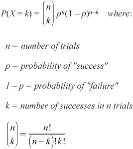
It’s important to note that many probability distributions do not fit a binomial setting, so it’s important that we can recognize when a distribution meets the four conditions of a binomial and when it does not. If a distribution meets the four conditions, we can use the shorthand notation, B(n, p), to represent a binomial distribution with n trials and probability of success equal to p. We sometimes call a binomial setting a Bernoulli trial. Once we have decided that a particular distribution is a binomial distribution, we can then apply the Binomial Probability Model. The formula for a binomial distribution is given on the AP* Statistics formula sheet.

Example 20: Consider Tess, a basketball player who consistently makes 70% of her free throws. Find the probability that Tess makes exactly 5 free throws in a game where she attempts 10 free throws. (We must make the assumption that the free throw shots are independent of one another.)

Solution: We can use the formula as follows:

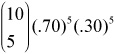There are 10 trials and we want exactly 5 trials to be a we want exactly 5 trials to be a “success.” means we have a combination of 10 things taken 5 at a time in any order. Some textbooks write this as ₁₀C₅. We can use our calculator to determine that there are in fact 252 ways to take 5 things from 10 things, if we do not care about the order in which they are taken. For example: Tess could make the first 5 shots and miss the rest. Or, she could make the first shot, miss the next 5, and then make the last 4. Or, she could make every other shot of the 10 shots. The list goes on. There are 252 ways she could make exactly 5 of the ten shots.

Notice that the probabilities of success and failure must add up to one since there are only two possible outcomes that can occur. Also notice that the exponents add up to 10. This is because we have 10 total trials with 5 successes and 5 failures.

We should be able to use our calculator to obtain:

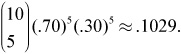
This is the work we would want to show on the AP* Exam!

We could also use the following calculator command on the TI 83/84: binompdf(10,.7,5). We enter 10 for the number of trials, .7 for the probability of success, and 5 as the number of trials we are going to obtain.

However, binompdf(10,.7,5) does not count as work on the AP* Exam.

You must show 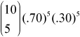even though you might not actually use it to get the answer. Binompdf is a calculator command specific to one type of calculator, not standard statistical notation. Don’t think you’ll get credit for writing down how to do something on the calculator. You will not! You must show the formula or identify the variable as a binomial as well as the parameters n and p.

Example 21: Consider the basketball player in Example 20. What is the probability that Tess makes at most 2 free throws in 10 attempts?

Solution: Consider that “at most 2” means Tess can make either 0, or 1, or 2 of her free throws. We write the following:

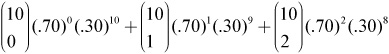
Always show this work.

We can either calculate the answer using the formula or use: binomcdf(10,.7,2) Notice that we are using cdf instead of pdf. The “c” in cdf means that we are calculating the cumulative probability. The graphing calculator always starts at 0 trials and goes up to the last number in the command. Again, the work you show should be the work you write when applying the formula, not the calculator command!

Either way we use our calculator we obtain:

Example 22: Again consider Example 20. What is the probability that Tess makes more than 2 of her free throws in 10 attempts?

Solution: Making more than 2 of her free throws would mean making 3 or more of the 10 shots. That’s a lot of combinations to consider and write down.

It’s easier to use the idea of the complement that we studied earlier in the chapter. Remember that if Tess shoots 10 free throws she could make anywhere between none and all 10 of her shots. Using the concept of the complement we can write:

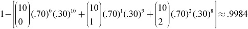
That’s pretty sweet. Try to remember this concept. It can make life a little easier for you!

Example 23: Find the expected number of shots that Tess will make and the standard deviation.

The following formulas are given on the AP* Exam:

Remember that the expected number is the average number of shots that Tess will make out of every 10 shots.

Thus, Tess will make 7 out of every 10 shots, on average. Seems logical!

Using the formula for standard deviation, we obtain:

Example 24: Consider Julia, a basketball player who consistently makes 70% of her free throws. What is the probability that Julia makes her first free throw on her third attempt?

How does this example differ from that of the previous section? In this example there are not a set number of trials. Julia will keep attempting free throws until she makes one. This is the major difference between binomial distributions and geometric distributions.

There are four conditions that must be met in order for a distribution to fit a geometric setting. These conditions are:

The probability that the first success is obtained in the nth observation is: P(X = n) = (1 − p)ⁿ⁻¹ p. Note that the smallest value that n can be is 1, not 0. The first success can happen on the first attempt or later, but there has to be at least one attempt. This formula is not given on the AP* Exam!

Returning to Example 24:

We want to find the probability that Julia makes her first free throw on her third attempt.

Applying the formula, we obtain:

We can either use the formula to obtain the answer or we can use:

Geompdf(0.7,3) Notice that we drop the first value that we would have used in binompdf, which makes sense because in a geometric probability we don’t have a fixed number of trials and that’s what the first number in the binompdf command is used for.

Once again, show the work for the formula, not the calculator command. No credit will be given for calculator notation.

Example 25: Using Example 24, what is the probability that Julia makes her first free throw on or before her fifth attempt?

Solution: This is again a geometric probability because Julia will keep shooting free throws until she makes one. For this problem, she could make the shot on her first attempt, second attempt, and so on until the fifth attempt. Applying the formula, we obtain:

or

We could also use the following formula, which is the formula for finding the probability that it takes more than n trials to obtain the first success:

Using this formula and the concept of the complement, we obtain:

Either method is OK as long as you show your work. If I used the first method, I would show at least three of the probabilities so that the grader of the AP* Exam knows that I understand how to apply the formula.

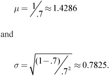
Example 26: Using Example 24, find the expected value (mean) and the standard deviation.

Solution: The mean in this case is the expected number of trials that it would take before the first success is obtained. The formulas for the mean and standard deviation are:

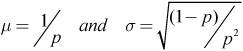
Applying these formulas (which are not given on the AP formula sheet), we obtain: