You will encounter certain types of sampling in AP Statistics. As always, it’s important that you fully understand all the concepts discussed in this chapter. We begin with some basic definitions.

A population is all the individuals in a particular group of interest. We might be interested in how the student body of our high school views a new policy about cell phone usage in school. The population of interest is all students in the school. We might take a poll of some students at lunch or during English class on a particular day. The students we poll are considered a sample of the entire population. If we sample the entire student body, we are actually conducting a census. A census consists of all individuals in the entire population. The U.S. Census attempts to count every resident in the United States and is required by the Constitution every ten years. The data collected by the U.S. Census will help determine the number of seats each state has in the House of Representatives. There has even been some political debate on whether or not the U.S. should spend money trying to count everyone when information could be gained by using appropriate sampling techniques.

A sampling frame is a list of individuals from the entire population from which the sample is drawn.

Several different types of sampling are discussed in AP Statistics. One type often referred to is an SRS, or simple random sample. An SRS is a sample in which every set of n individuals has an equal chance of being chosen. Referring back to our population of students, we could conduct an SRS of size 100 from the 2200 students by numbering all students from 1 to 2200. We could then use the random integer function on our calculator, or the table of random digits, or we could simply draw 100 numbers out of a hat that included the 2200 numbers. It’s important to note that, in an SRS, not only does every individual in the population have an equal opportunity of being chosen, but so does each sample.

When using the table of random digits, we should remember a few things. First of all, there are many different ways to use the table. We’ll discuss one method and then I’ll briefly give a couple examples of another way that the table might be used. Consider our population of 2200 students. After numbering each student from 0001 to 2200, we can go to the table of random digits (found in many statistics books). We can go to any line—let’s say line 145. We can look at the first four-digit number, which is 1968. This would be the first student selected for our sample. The next number is 7126. Since we do not have a student numbered 7126, we simply skip over 7126. We also skip 3357, 8579, and 5806. The next student chosen is 0993. We continue in this fashion until we’ve selected the number of students we want in our sample. If we get to the end of the line, we simply go on the next line. This is only one method we could use. A different method might be to start at the top with line 101. Use the first “chunk” of five digits and use the last four digits of that five-digit number (note that the numbers are grouped in groups of five for the purpose of making the table easier to read). That would give us 9223, which we would skip. We could then either go across to the next “chunk” of five digits or go down to the “chunk” of five digits below our first group. No matter how you use the random digit table, just remember to be consistent and stay with the same system until the entire sample has been chosen. Skipping the student numbered 1559 because he’s your old boyfriend or she’s your old girlfriend is not what random sampling is all about.

A stratified random sample could also be used to sample our student body of 2200 students. We might break up our population into groups that we believe are similar in some fashion. Maybe we feel that freshmen, sophomores, juniors, and seniors will feel different about our new policy concerning cell phones. We call these homogeneous groups strata. Within each stratum, we would then conduct an SRS. We would then combine these SRSs to obtain the total sample. Stratified random sampling guarantees representation from each strata. In other words, we know that our sample includes the opinions of freshmen, sophomores, juniors, and seniors.

A cluster sample is similar to a stratified sample. In a cluster sample, however, the groups are heterogeneous, not homogeneous. That is, we don’t feel like the groups will necessarily differ from one another. Once the groups are determined, we can conduct an SRS within each group and form the entire sample from the results of each SRS. Usually this method is used to make the sampling cheaper or easier. We might sample our 2200 students during our three lunch periods. We could form three SRSs from our three lunch groups as long as we feel that all three lunch groups are similar to one another and all represent the population equally.

Systematic sampling is a method in which it is predetermined how the sample will be obtained. We might, for example, sample every 25^th student from our list of 2200 students. We should note that this method is not considered an SRS since not all samples of a given size have an equal chance of being chosen. Think about it this way: If we sample every 25^th student of the 2200, that’s 88 students. The first 25 students on the list of the 2200 students would never be chosen together, so technically it’s not an SRS.

A convenience sample could also be conducted from our 2200 students. We would conduct a convenience sample because it’s, well, convenient. We might sample students in the commons area near the cafeteria because it’s an easy thing to do and we can do so during our lunch break. It should be noted, however, that convenience samples almost always contain bias. That is to say that they tend to systematically understate or overstate the proportion of people that feel a certain way; they are usually not representative of the entire population.

A voluntary response sample could be obtained by having people respond on their own. We might try to sample some of our 2200 students by setting up an online survey where students could respond one time to a survey if they so choose. These types of samples suffer from voluntary response bias because those that feel very strongly either for or against something are much more willing to respond. Those that feel strongly against something are actually more likely to respond than those that have strong positive feelings.

A multistage sample might also be used. This is sampling that combines several different types of sampling. Some national opinion polls are conducted using this method.

We should also be concerned with how survey questions are worded. We should ensure that the wording is not slanted in such a way as to sway the person taking the survey to answer the question in a particular manner. Poorly worded questions can lead to response bias. Training sometimes takes place so that the person conducting the survey interview uses good interviewing techniques.

Undercoverage occurs when individuals in the population are excluded in the process of choosing the sample. Undercoverage can lead to bias, so caution must be used.

Nonresponse can also lead to bias when certain selected individuals cannot be reached or choose not to participate in the sample.

Our goal is to eliminate bias. Through proper sampling, it is possible to eliminate a good deal of the bias that can be present if proper sampling is not used. We must realize that sampling is never perfect. If I draw a sample from a given population and then draw another sample in the exact same manner, I rarely get the exact same results. There is almost always some sampling variability. Think about sampling our student body of 2200 students. If we conduct an SRS of 25 students and then conduct another SRS of 25 students, we will probably not be sampling the same 25 students and thus may not get the exact same results. More discussion about sampling viability will take place in later chapters. Remember, however, that larger random samples will give more accurate results than smaller samples conducted in the same manner. A smaller random sample, however, may give more accurate results than a larger non-random sample.

Now that we’ve discussed some different types of sampling, it’s time to turn our attention to experimental design. It’s important to understand both observational studies and experiments and the difference between them. In an observational study, we are observing individuals. We are studying some variable about the individuals but not imposing any treatment on them. We are simply studying what is already happening. In an experiment, we are actually imposing a treatment on the individuals and studying some variable associated with that treatment. The treatment is what is applied to the subjects or experimental units. We use the term “subjects” if the experimental units are humans. The treatments may have one or more factors, and each factor may have one or more levels.

Example 1: Consider an experiment where we want to test the effects of a new laundry detergent. We might consider two factors: water temperature and laundry detergent. The first factor, temperature, might have three levels: cold, warm, and hot water. The second factor, detergent, might have two levels: new detergent and old detergent. We can combine these to form six treatments as listed in Figure 4.1.

Figure 4.1. Six treatments.

It’s important to note that we cannot prove or even imply a cause-and-effect relationship with an observational study. We can, however, prove a cause-and-effect relationship with an experiment. In an experiment, we observe the relationship between the explanatory and response variables and try to determine if a cause-and-effect relationship really does exist.

The first type of experiment that we will discuss is a completely randomized experiment. In a completely randomized experiment, subjects or experimental units are randomly assigned to a treatment group. Completely randomized experiments can be used to compare any number of treatments. Groups of equal size should be used, if possible.

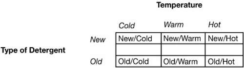
Example 2: Consider an experiment in which we wish to determine the effectiveness of a new type of arthritis medication. We might choose a completely randomized design. Given 600 subjects suffering from arthritis, we could randomly assign 200 subjects to group 1, which would receive the new arthritis medication, 200 subjects to group 2, which would receive the old arthritis medication, and 200 subjects to group 3, which would receive a placebo, or “dummy” pill. To ensure that the subjects were randomly placed into one of the three treatment groups, we could assign each of the 600 subjects a number from 001 to 600. Using the random integer function on our calculator, we could place the first 200 subjects whose numbers come up in group 1, the second 200 chosen in group 2, and the remaining subjects in group 3. It should be noted that a placebo is used to help control the placebo effect, which comes into play when people respond to the “idea” that they are receiving some type of treatment. A placebo, or “dummy” pill, is used to ensure that the placebo effect contributes equally to all three groups. The placebo should taste, feel, and look like the real medication. The subjects would take the medication for a predetermined period of time before the effectiveness of the medication was evaluated. We can use a diagram to help outline the design (see Figure 4.2).

Figure 4.2. A completely randomized design.

To describe an experiment, it can be useful (but not essential) to use a diagram. Remember to explain how you plan to randomly assign individuals to each treatment in the experiment. This can be as simple as using the table of random digits or using the random integer function of the graphing calculator. Be specific in your diagram, and be sure to fully explain how you are setting up the experiment.

Example 3: Let’s reconsider Example 2. Suppose there is reason to believe that the new arthritis medication might be more effective for men than for women. We would then use a type of design called a block design. We would divide our group of 600 subjects into one group of males and one group of females. Once our groups were blocked on gender, we would then randomly assign our group of males to one of the three treatment groups and our group of females to one of the three treatment groups. It’s important to note that the use of blocking reduces variability within each of the blocks. That is, it eliminates a confounding variable that may systematically skew the results. For example, if one is conducting an experiment on a weight-loss pill and blocking is not used, the random assignment of the subjects may assign more females to the experimental group. If males and females respond differently to the treatment, you will not be able to determine whether the weight loss is due to the drug’s effectiveness or due to the gender of the subjects in the group. Be sure to include random assignment in your diagram, but make sure that you’ve done so after you’ve separated males and females. There are often a few students who get in a hurry on an exam and randomly place subjects into groups of males and females. It’s good that they remember that random assignment is important, but it needs to come after the blocking, not before.

The arthritis experiment in Examples 2 and 3 might be either a single-blind or double-blind experiment. In a single-blind experiment, the person taking the medication would not know whether they had the new medication, the old medication, or the placebo. If a physician is used to help assess the effectiveness of the treatments, the experiment should probably be double-blind. That is, neither the subject receiving the treatment nor the physician would know which treatment the subject had been given. Obviously, in the case of a double-blind experiment, there must be a third-party member that knows which subjects received the various treatments.

Example 4: A manufacturer of bicycle tires wants to test the durability of a new material used in bicycle tires. A completely randomized design might be used where one group of cyclists uses tires made with the old material and another group uses tires made with the new material. The manufacturer realizes that not all cyclists will ride their bikes on the same type of terrain and in the same conditions. To help control for these variables, we can implement a matched-pairs design. Matching is a form of blocking. One way to do this is to have each cyclist use both types of tires. A coin toss could determine whether the cyclist uses the tire with the new material on the front of the bike or on the rear. We could then compare the front and rear tire for each cyclist. Another way to match in this situation might be to pair up cyclists according to rider size and weight, the location where they ride, and/or the type of terrain they typically ride on. A coin could then be tossed to decide which of the two cyclists uses the tires with the new material and which uses the tires with the old material. This method might not be as effective as having each cyclist serve as his/her own control and use one tire of each type.

When you’re designing various types of experiments, it’s important to remember the four principles of experimental design. They are:

Simulation can be used in statistics to model random or chance behavior. In much the same way an airplane simulator models how an actual aircraft flies, simulation can be used to help us predict the probability of some real-life occurrences. For our purposes in AP Statistics, we’ll try to keep it simple. If you are asked to set up a simulation in class or even on an exam, keep it simple. Use things like the table of random digits, a coin, a die, or a deck of cards to model the behavior of the random phenomenon.

Let’s set up an example: As I was walking out of the grocery store a few years ago, my two children, Cassidy and Nolan (ages 5 and 7 at the time), noticed a lottery machine that sold “scratch-offs” near the exit of the store. Despite explaining to them how the “scratch-offs” worked and that the probability of winning was, well … not so good, they persuaded me to partake in the purchase of three $1 “scratch-offs.” Being an AP Stats teacher and all, I knew I had a golden opportunity to teach them a lesson in probability and a “lesson” that gambling was “risky business.”

Sure, we might win a buck or two, but chances were pretty good that we’d lose, and even if we did win, the kids would hopefully lose interest since we would most likely just be getting our money back. Once we were in the car, the lesson began. “Hmmm …“Odds are 1:4,” I told them. That means that on average, you win about one time for every five times you play. I carefully explained that the chances of winning were not very good and that if we won, chances were pretty good that we would not win a lot. Two “scratch-offs” later … two winners, $1 each. Hmmm.… Not exactly what I had planned, but at least I had my $2 back. “Can we buy some more?” they quickly asked. I told them that the next time we stopped for gas, we could buy two more “scratch-offs” but that was it. Surely they’d learn their lesson this time. Two weeks later, we purchased two more $1 “scratch-offs.” Since I was in a hurry, I handed each of them a coin and a “scratch-off” and away we drove. Unfortunately for Nolan, his $1 “scratch off” resulted in a loss. I felt a little bad about his losing, but in the long run it would probably be best. Moments later, Cassidy yells out, “I won a hundred dollars!” Sure, I thought. She’s probably just joking. “Let me see that!” I quickly pulled over at the next opportunity to realize that she had indeed won $100! Again, not exactly what I’d planned, but hey … it was $100! What are the chances of winning on three out of four “scratch-offs?” Let’s set up a simulation to try to answer the question.

Example 5: Use simulation to find the probability that someone who purchases four $1 “scratch-offs” will win something on three out of the four “scratch-offs.” Assume the odds of winning on the “scratch-off” are 1:4.

Solution: If the odds of winning are 1:4, that means that in the long run we should expect to win one time out of every five plays. That is, we should expect, out of five plays, to win once and lose four times, on average. In other words, the probability of winning is 1/5. Sometimes we might win more than expected and sometimes we might win less than expected, but we should average one win for every four losses. We can set up a simulation to estimate the probability of winning.

Note that 0–1 is actually 2 numbers and 2–9 is 8 numbers. Also note that 1:4 odds would be the same as 2:8 odds. We have used single-digit numbers for the assignment as it is the simplest method in this case. We could have used double-digit numbers for the assignment, but this would be unnecessary. Several different methods would work as long as the odds reduce to 1:4. To make it easier to keep track of the numbers, we will group the one-digit numbers in “chunks” of four and label each group “W” for win and “L” for lose. Each group of four one-digit numbers represents one simulation of purchasing four “scratch-offs” (Figure 4.3). Starting at line 107 of the table of random digits, we obtain:

Figure 4.3 displays 50 trials of purchasing four “scratch-off” tickets. Only one of the 50 trials produced three winning tickets out of four. Based on our simulation, the probability of winning three out of four times is only 1/50. In other words, Cassidy and Nolan were pretty lucky. Students sometimes find simulation to be a little tricky. Remember to keep it as simple as possible. A simulation does not need to be complicated to be effective.