3.1 Density Curves
3.2 Normal Distributions
3.3 Normal Calculations
![]() Density curves are smooth curves that can be used to describe the overall pattern of a distribution. Although density curves can come in many different shapes, they all have something in common: The area under any density curve is always equal to one. This is an extremely important concept that we will utilize in this and other chapters. It is usually easier to work with a smooth density curve than a histogram, so we sometimes overlay the density curve onto the histogram to approximate the distribution. A specific type of density curve called a normal curve will be addressed in section 3.2. This “bell-shaped” curve is especially useful in many applications of statistics as you will see later on. We describe density curves in much the same way we describe distributions when using graphs such as histograms or stemplots.
Density curves are smooth curves that can be used to describe the overall pattern of a distribution. Although density curves can come in many different shapes, they all have something in common: The area under any density curve is always equal to one. This is an extremely important concept that we will utilize in this and other chapters. It is usually easier to work with a smooth density curve than a histogram, so we sometimes overlay the density curve onto the histogram to approximate the distribution. A specific type of density curve called a normal curve will be addressed in section 3.2. This “bell-shaped” curve is especially useful in many applications of statistics as you will see later on. We describe density curves in much the same way we describe distributions when using graphs such as histograms or stemplots.
![]() The relationship between the mean and the median is an important concept, especially when dealing with density curves. In a symmetrical density curve, the mean and median will be equal if the distribution is perfectly symmetrical or approximately equal if the distribution is approximately symmetrical. If a distribution is skewed left, then the mean will be “pulled” in the direction of the skewness and will be less than the median. If a distribution is skewed right, the mean is again “pulled” in the direction of the skewness and will be greater than the median. Figure 3.1 displays distributions that are skewed left, skewed right, and symmetrical. Notice how the mean is “pulled” in the direction of the skewness.
The relationship between the mean and the median is an important concept, especially when dealing with density curves. In a symmetrical density curve, the mean and median will be equal if the distribution is perfectly symmetrical or approximately equal if the distribution is approximately symmetrical. If a distribution is skewed left, then the mean will be “pulled” in the direction of the skewness and will be less than the median. If a distribution is skewed right, the mean is again “pulled” in the direction of the skewness and will be greater than the median. Figure 3.1 displays distributions that are skewed left, skewed right, and symmetrical. Notice how the mean is “pulled” in the direction of the skewness.
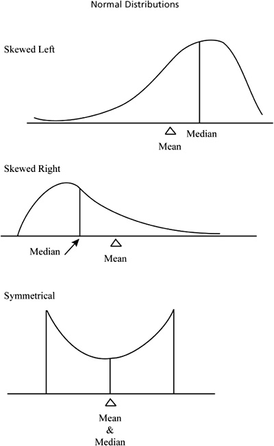
![]() It’s important to remember that the mean is the “balancing point” of the density curve or histogram and that the median divides the density curve or histogram into two parts, equal in area (Figure 3.2).
It’s important to remember that the mean is the “balancing point” of the density curve or histogram and that the median divides the density curve or histogram into two parts, equal in area (Figure 3.2).
The mean is the balancing point. The median divides the area into two equal parts.

![]() One particular type of density curve that is especially useful in statistics is the normal curve, or normal distribution. Although all normal distributions have the same overall shape, they do differ somewhat depending on the mean and standard deviation of the distribution (Figure 3.3). If we increase or decrease the mean while keeping the standard deviation the same, we will simply shift the distribution to the right or to the left. The more we increase the standard deviation, the “wider” and “shorter” the density curve will be. If we decrease the standard deviation, the density curve will be “narrower” and “taller.” Remember that all density curves, including normal curves, have an area under the curve equal to one. So, no matter what value the mean and standard deviation take, the area under the normal curve is equal to one. This is very important, as you’ll soon see.
One particular type of density curve that is especially useful in statistics is the normal curve, or normal distribution. Although all normal distributions have the same overall shape, they do differ somewhat depending on the mean and standard deviation of the distribution (Figure 3.3). If we increase or decrease the mean while keeping the standard deviation the same, we will simply shift the distribution to the right or to the left. The more we increase the standard deviation, the “wider” and “shorter” the density curve will be. If we decrease the standard deviation, the density curve will be “narrower” and “taller.” Remember that all density curves, including normal curves, have an area under the curve equal to one. So, no matter what value the mean and standard deviation take, the area under the normal curve is equal to one. This is very important, as you’ll soon see.

The equation for the standard normal curve is: ![]()
![]() All normal distributions follow the Empirical Rule. That is to say that all normal distributions have: 68% of the observations falling within σ (one standard deviation) of the mean, 95% of the observations falling within 2σ (two standard deviations) of the mean, and 99.7% (almost all) of the observations falling within 3σ (three standard deviations) of the mean (Figure 3.4).
All normal distributions follow the Empirical Rule. That is to say that all normal distributions have: 68% of the observations falling within σ (one standard deviation) of the mean, 95% of the observations falling within 2σ (two standard deviations) of the mean, and 99.7% (almost all) of the observations falling within 3σ (three standard deviations) of the mean (Figure 3.4).
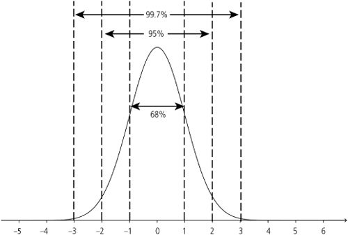
Figure 3.4. About 68% of observations fall within one standard deviation, 95% within two standard deviations, and 99.7% within three standard deviations.
![]() Example 1: Let’s assume that the number of miles that a particular tire will last roughly follows a normal distribution with μ = 40,000 miles and σ = 5000 miles. Note that we can use shorthand notation N(40,000, 5000) to denote a normal distribution with mean equal to 40,000 and standard deviation equal to 5,000. Since the distribution is not exactly normal but approximately normal, we can assume the distribution will roughly follow the 68, 95, 99.7 Rule. Using the 68, 95, 99.7 Rule we can conclude the following (see Figure 3.5):
Example 1: Let’s assume that the number of miles that a particular tire will last roughly follows a normal distribution with μ = 40,000 miles and σ = 5000 miles. Note that we can use shorthand notation N(40,000, 5000) to denote a normal distribution with mean equal to 40,000 and standard deviation equal to 5,000. Since the distribution is not exactly normal but approximately normal, we can assume the distribution will roughly follow the 68, 95, 99.7 Rule. Using the 68, 95, 99.7 Rule we can conclude the following (see Figure 3.5):
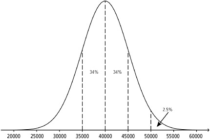
About 68% of all tires should last between 35,000 and 45,000 miles (μ ± σ)
About 95% of all tires should last between 30,000 and 50,000 miles (μ ± 2σ)
About 99.7% of all tires should last between 25,000 and 55,000 miles (μ ± 3σ)
Using the 68, 95, 99.7 Rule a little more creatively, we can also conclude:
About 34% of all tires should last between 40,000 and 45,000 miles.
About 34% of all tires should last between 35,000 and 40,000 miles.
About 2½% of all tires should last more than 50,000 miles.
About 84% of all tires should last less than 45,000 miles.
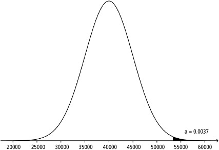
![]() Example 2: Referring back to Example 1, let’s suppose that we want to determine the percentage of tires that will last more than 53,400 miles. Recall that we were given N(40,000, 5000). To get a more exact answer than we could obtain using the Empirical Rule, we can do the following:
Example 2: Referring back to Example 1, let’s suppose that we want to determine the percentage of tires that will last more than 53,400 miles. Recall that we were given N(40,000, 5000). To get a more exact answer than we could obtain using the Empirical Rule, we can do the following:
Solution: Always make a sketch! (See Figure 3.6.)
Shade the area that you are trying to find, and label the mean in the center of the distribution. Remember that the mean and median are equal in a normal distribution since the normal curve is symmetrical.
Obtain a standardized value (called a z-score) using ![]()
Notice that the formula for z takes the difference of x and μ and divides it by σ. Thus, a z-score is the number of standard deviations that x lies above or below the mean. So, 53,400 is 2.68 standard deviations above the mean. You should always get a positive value for z if the value of x is above the mean, and a negative value for z if the value of x is below the mean.
When we find the z-score, we are standardizing the values of the distribution. Since these values are values of a normal distribution, the distribution we obtain is called the standard normal distribution. This new distribution, the standard normal distribution, has a mean of zero and a standard deviation of one. We can then write N(0,1)
The advantage of standardizing any given normal distribution to the standard normal distribution is that we can now find the area under the curve for any given value of x that is needed.
We can now use the z-score of 2.68 that we obtained earlier. Using Table A, we can look up the area to the left of z = 2.68. Notice that Table A has two sides—one for positive values for z and the other for negative values for z. Using the side of the table with the positive values for z, follow the left-hand column down until you reach 2.6. Then go across the top of the table until you reach .08. By cross-referencing 2.6 and .08, we can obtain the area to the left of z = 2.68, which is 0.9963.
In other words, 99.63% of tires will last less than 53,400 miles. We want to know what percent of tires will last more than 53,400 miles, so we subtract 0.9963 from 1. Remember that the total area under any density curve is equal to one.
We obtain 1 − 0.9963 = 0.0037.
That is, only 0.37% of tires will last more than 53,400 miles. We can also state that the probability that a randomly chosen tire of this type will last longer than 53,400 miles is equal to 0.0037.
![]() Example 3: Again referring to Example 1, find the probability that a randomly chosen tire will last between 32,100 miles and 41,900 miles.
Example 3: Again referring to Example 1, find the probability that a randomly chosen tire will last between 32,100 miles and 41,900 miles.
Make a sketch. (See Figure 3.7.)

Locate the mean on the normal curve as well as the values of 32,100 and 41,900. Shade the area between 32,100 and 41,900.
Calculate the z-scores.
Find the areas to the left of −1.58 and 0.38 using Table A.
The area to the left of −1.58 is equal to 0.0571, and the area to the left of 0.38 is equal to 0.6480.
Since we want to know the probability that a tire will last between 32,100 and 41,900 miles, we will subtract the two areas. Remember that any area that we look up in Table A is the area to the left of z.
0.6480 − 0.0571 = 0.5909
Conclude in context:
The probability that a randomly chosen tire will last between 32,100 miles and 41,900 miles is equal to 0.5909.
![]() Example 4: Consider a national mathematics exam where the distribution of test scores roughly follows a normal distribution with mean, μ = 320, and standard deviation, μ = 32. What score must a student obtain to be in the top 10% of all students taking the exam?
Example 4: Consider a national mathematics exam where the distribution of test scores roughly follows a normal distribution with mean, μ = 320, and standard deviation, μ = 32. What score must a student obtain to be in the top 10% of all students taking the exam?
Make a sketch! (See Figure 3.8.)
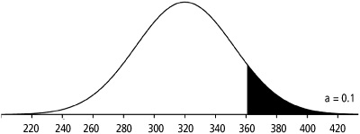
Shade the appropriate area.
Use the formula for z.
Using substitution, we obtain:
In order to solve for x, we need to obtain an appropriate value of z. Using Table A “backwards,” we look in the body of the table for the value closest to 0.90, which is 0.8997. The value of z that corresponds to an area to the left of 0.8997 is 1.28, so z = 1.28. Again, remember that everything we look up in Table A is the area to the left of z, so we look up what’s closest to 0.90, not 0.10.
Substituting for z, we obtain:
Solving for x, we obtain:
x = 360.96
Conclude in context.
A student must obtain a score of approximately 361 in order to be in the top 10% of all students taking the exam.
![]() Example 5: Consider the national mathematics test in Example 4. The middle 90% of students would score between which two scores?
Example 5: Consider the national mathematics test in Example 4. The middle 90% of students would score between which two scores?
Make a sketch! (See Figure 3.9.)
Shade the appropriate area.
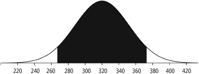
Use the formula for z.
Using substitution, we obtain:
In order to solve for x, we need to obtain an appropriate value of z. Consider that we are looking for the middle 90% of test scores. Remembering once again that the area under the normal curve is 1, we can obtain the area on the “outside” of 90%, which would be 10%. This forms two “tails,” which we consider the right and left tails.
These “tails” are equal in area and thus have an area of 0.05 each. We can then use Table A, as we did in Example 4, to obtain a z-score that corresponds to an area of 0.05. Notice that two values are equidistant from 0.05. These areas are 0.0495 and 0.0505, which correspond to z-scores of −1.64 and −1.65, respectively. Since the areas we are looking up are the same distance away from 0.05, we split the difference and go out one more decimal place for z. We use z = −1.645.
Solving for x, we obtain:
x = 267.36
We can now find the test score that would be the cutoff value for the top 5% of scores. Notice that since the two tails have the same area, we can use z = 1.645. The z-scores are opposites due to the symmetry of the normal distribution.
Solving for x, we obtain:
x = 372.64
Conclude in context.
The middle 90% of students will obtain test scores that range from approximately 267 to 373.
![]() Inferential statistics is a major component of the AP Statistics curriculum. When you infer something about a population based on sample data, it is often important to assess the normality of a population. We can do this by looking at the number of observations in the sample that lie within one, two, and three standard deviations from the mean. In other words, use the Empirical Rule. Do approximately 68, 95, and 99.7% of the observations fall within μ ± 1σ, μ ± 2σ, and μ ± 3σ? Larger data sets should roughly follow the 68, 95, 99.7 Rule while smaller data sets typically have more variability and therefore may be less likely to follow the Empirical Rule despite coming from normal populations.
Inferential statistics is a major component of the AP Statistics curriculum. When you infer something about a population based on sample data, it is often important to assess the normality of a population. We can do this by looking at the number of observations in the sample that lie within one, two, and three standard deviations from the mean. In other words, use the Empirical Rule. Do approximately 68, 95, and 99.7% of the observations fall within μ ± 1σ, μ ± 2σ, and μ ± 3σ? Larger data sets should roughly follow the 68, 95, 99.7 Rule while smaller data sets typically have more variability and therefore may be less likely to follow the Empirical Rule despite coming from normal populations.
![]() We can also look at a graph of the sample data. By constructing a histogram, stemplot, modified boxplot, or line plot, we can examine the data to look for strong skewness and outliers. Non-normal populations often produce sample data that have skewness or outliers or both. Normal populations are more likely to have sample data that are symmetrical and bell-shaped and usually do not have outliers.
We can also look at a graph of the sample data. By constructing a histogram, stemplot, modified boxplot, or line plot, we can examine the data to look for strong skewness and outliers. Non-normal populations often produce sample data that have skewness or outliers or both. Normal populations are more likely to have sample data that are symmetrical and bell-shaped and usually do not have outliers.
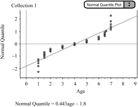
![]() Normal probability plots can also be used to assess the normality of a population through sample data. A normal probability plot is a scatterplot that graphs a predicted z-score against the value of the variable. Most graphing calculators and statistical software packages are capable of constructing normal probability plots. You should be much more concerned with how to interpret a normal probability plot than with how one is constructed. Again, technology helps us out in constructing the plot.
Normal probability plots can also be used to assess the normality of a population through sample data. A normal probability plot is a scatterplot that graphs a predicted z-score against the value of the variable. Most graphing calculators and statistical software packages are capable of constructing normal probability plots. You should be much more concerned with how to interpret a normal probability plot than with how one is constructed. Again, technology helps us out in constructing the plot.
![]() Interpret the normal probability plot by assessing the linearity of the plot. The more linear the plot, the more normal the distribution. A non-linear probability plot is a good sign of a non-normal population. Consider the following data taken from a distribution known to be uniform and non-normal (Figure 3.10). The accompanying normal probability plot is curved and is thus a sign that the data is indeed taken from a non-normal population.
Interpret the normal probability plot by assessing the linearity of the plot. The more linear the plot, the more normal the distribution. A non-linear probability plot is a good sign of a non-normal population. Consider the following data taken from a distribution known to be uniform and non-normal (Figure 3.10). The accompanying normal probability plot is curved and is thus a sign that the data is indeed taken from a non-normal population.