Applying Financial Models: To Value, Structure, and Negotiate Stock and Asset Purchases
Abstract
In this chapter, the focus is on the application of financial modeling to value and structure mergers and acquisitions (M&As). A detailed discussion of how to construct M&A financial models is beyond the scope of this chapter. Rather, the intent of this chapter is to provide the reader with an appreciation of the general characteristics of such models, their data input requirements, and how they may be used to address questions relating to valuation, deal structuring, and financing, as well as their limitations. For example, models help an acquirer determine the implications of various possible deal structures before submitting an initial offer and in assessing the implications of various financing or postclosing capital structures. However, caution is required when assessing model outputs as they can be manipulated to reflect the biases of their users. Both acquirers and target firms can use models to evaluate rapidly alternative proposals and counterproposals likely to arise during the negotiation process. Models also help all parties to the transaction understand the key determinants of value and the relative contribution of each party to value creation. Such information is critical to each side in the negotiating process in determining an appropriate purchase price and distribution of risk. This chapter also describes in detail how to quantify synergy, the mechanics of estimating the value of options, warrants, and convertible securities in the context of financial modeling, lists common sources of data used in the modeling process, financial statement illustrations, model workflow diagrams, and the logic underlying offer price determination.
Keywords
M&A deal structuring; M&A negotiation; M&A transactions; Negotiating deals; Merger valuation; Deal structuring; Financial models; M&A models; M&A valuation; Financing M&As; Offer price determination; Capital structure; Model simulation; Assessing alternative deal structures; Synergy; Fully diluted shares; Share exchange ratios; Earnings per share; Cost of capital; Valuation; Revenue-related synergy; Cost-related synergy; Stock purchases; Asset purchases; Cost of equity; CAPM; Capital asset pricing model; Deal negotiation; Deal financing; Deal structuring; Value drivers; Model assumptions; Standalone value; Deal terms; Asset purchases; Stock purchases; Options; Warrants; Convertible securities; Revolving loan facilities
He who lives by the crystal ball soon learns to eat ground glass.
Edgar R. Fiedler
Inside M&A: The Anatomy of a M&A Negotiation
Sometimes portrayed as America’s healthiest food store, Whole Foods Market Inc. (Whole Foods) was founded in 1978. Its business strategy is one of a generic differentiation in which it distinguishes itself from competitors by a focus on organic or natural products. The firm promotes product quality by securing suppliers able and willing to adhere to its high quality standards. The firm grows through increasing market share organically by opening up new stores and by offering new products to attract additional customers.
What would be the likely long-term impact of such a strategy? Sophisticated firms typically utilize long range planning as described in Chapters 4 and 5 to evaluate their ability to perform in their future competitive environment. Financial models are commonly used to project a “baseline” forecast or reference projection of cash flow over a number of years to determine if the firm’s current strategy results in achieving its vision and long-term goals.
In developing its baseline financial model projection, Whole Foods had to make numerous assumptions about the future. These could have included consumer income growth, responsiveness of consumers to rising retail food prices, rivals increased offering of organic foods, increasing wholesale food prices, and higher labor costs due to rising state minimum wage statutes and a tightening labor market. Additional fixed expenses like depreciation and financing costs would have to be considered, as well as the cost of opening new stores. Based on these assumptions, the model would estimate the firm’s market value, operating cash flows, earnings per share, and other financial metrics. The baseline projection can subsequently be adjusted for alternative scenarios ranging from accelerated investment to the outright sale of the firm. That scenario offering the highest net present value should be selected to maximize shareholder value.
By early 2017, Whole Foods, long a Wall Street darling, had seen its shares fall by half since its all-time high in October 2013. The firm was being whipsawed by aggressive competition from Kroger and Wal-Mart, as well as from Amazon.com and startups like Blue Apron. Impatient with the pace of the firm’s turnaround efforts, activist investor Jana Partners (which had a 9% ownership stake in the upscale grocer) in mid-April 2017 pushed the firm to accelerate efforts to turnaround its performance. Threatened with a proxy fight to restructure the board, Whole Foods argued it needed more time for its business strategy to achieve the expected results. With same store sales continuing to decline, Jana was unimpressed, ultimately forcing the board to investigate what the firm would be worth if sold. Consequently, Whole Foods hired an investment bank to market the sale of the entire firm to selected parties.
Seven firms including two industry competitors, four private equity firms, and Amazon.com expressed interest in Whole Foods. During the next several weeks, Whole Foods’ management weighed its options. One competing grocery retailer suggested a “merger of equals,” while another wanted to negotiate a long-term supply contract. The board and senior management and their advisors poured over financial spreadsheets to evaluate the alternative offers.
Amazon.com made its initial all-cash bid of $41 per share for the firm in early May 2017 and insisted that the negotiations be secret to avoid an auction for the business. Amazon nearly walked away after Whole Foods made a counter-offer of $45 per share. The two firms finally reached agreement in early July 2017 in a deal valued at $13.7 billion or $42 per share, well above the firm’s exchange-listed share price of $35. Immediately following the announcement, Whole Foods shares soared as investors were expecting higher bids from rivals. In reality, the other six bidders had been shut out of the process. A week later the firm’s share price plummeted as investors realized that no additional bidders would emerge.
Not only would Whole Foods have used financial models to evaluate offers, the bidders would have employed models to determine potential synergies and how long it would take to earn back a purchase price premium and still earn their cost of capital. Whole Foods could have used models to provide their own estimate of potential synergy, arguing their shareholders should be compensated for the amount of value they are contributing to the merged firms.
Thus, from start to finish, financial models can play a key role in the M&A process. For Whole Foods, models provide a baseline projection reflecting its current strategy, the ability to evaluate alternative ways of maximizing shareholder value, and a means of assessing the relative merits of various bids. For Amazon.com, financial models would help determine an appropriate offer price for Whole Foods that would enable Amazon to earn its cost of capital.
Chapter Overview
As illustrated in Amazon.com’s takeover of Whole Foods case study, financial models are commonly used in various aspects of the M&A process. The emphasis in Chapter 9 was on how financial modeling can be used to estimate the standalone value of a single firm. In this chapter, the focus is on the application of financial modeling to value and structure mergers and acquisitions. A detailed discussion of how to construct M&A financial models is beyond the scope of this book. Rather, the intent of this chapter is to provide the reader with an appreciation of the general characteristics of such models, their data input requirements, and how they may be used to address questions relating to valuation, deal structuring, and financing (Table 14.1). Such information is critical to each side in the negotiating process in determining an appropriate purchase price and distribution of risk.
Table 14.1
| Key questions • Valuation (see Chapters 7 and 8) – What are the key drivers of firm value? – How much is Target worth without the effects of synergy (i.e., standalone value)? How much is Acquirer worth on a standalone basis? Will the combination of the two businesses create value for Acquirer’s shareholders? – What is the value of expected synergy? – What is the maximum price Acquirer should pay for Target? • Financing (see Chapter 13) – Can the proposed purchase price be financed? – What combination of potential sources of funds, both internally generated and external sources, provides the lowest cost of funds for Acquirer, subject to existing loan covenants and credit ratios Acquirer hopes to maintain or achieve? – What is the acquisition’s impact on Acquirer’s fully diluted earnings per share? – Are existing loan covenants violated? – Is the firm’s credit rating in jeopardy? – Will the firm’s ability to finance future opportunities be impaired? • Deal structuring (see Chapters 11 and 12) – What is the impact on financial performance and valuation if Acquirer is willing to assume certain Target liabilities? – What is the impact on Acquirer’s earnings per share of alternative forms of payment? – What are the implications of a purchase of stock versus a purchase of assets? – What is the distribution of ownership of the combined businesses between Acquirer and Target shareholders following closing? – What is the impact on Acquirer’s financial performance of a tax free rather than a taxable deal? |

This chapter begins with a discussion of elements common to most sophisticated M&A financial models, followed by illustrations of how M&A models may be applied to a purchase of stock and a purchase of assets. The acquiring firm, target firm, and combined firms are referred to throughout the chapter as Acquirer, Target, and Newco, respectively. The case study at the end of this chapter provides a hypothetical illustration of how models could have been applied in the negotiation process using a completed deal in which lab equipment maker Thermo Fisher Scientific Inc. merged with Life Technologies Corporation. See Appendix A for a listing of potential sources of data inputs required to run the financial model discussed in this chapter.
The Excel worksheets of the detailed M&A model discussed in this chapter are available on the companion site to this book in a Microsoft Excel file entitled M&A Valuation and Deal Structuring Model (https://www.elsevier.com/books-and-journals/book-companion/9780128150757). A review of this chapter also is available in the file folder entitled “Student Study Guide” on the companion site.
Understanding and Applying M&A Financial Models
The logic underlying the Excel-based M&A model found on the companion site follows the four step process outlined in (Table 14.2). The key outputs of the model for a purchase of stock deal are displayed on Acquirer Transaction Summary Worksheet (Table 14.3). This table allows for a quick review of deal terms and their implications based on specific assumptions. The cells highlighted in yellow are called “input cells” and require the analyst to input data. The remaining cells have formulas utilizing these inputs to calculate their values automatically.
Table 14.2


Common Elements of M&A Models
M&A models commonly require the estimation of the standalone value of Target and Acquirer. The standalone value is what the firm would be worth if it were an independent entity and all revenue is valued at current market prices and all costs incurred in generating these revenues are known. The standalone value of Target is theoretically what the business would be worth in the absence of any takeover bid; Acquirer’s standalone value represents a reference point against which the value of the combined businesses (Newco) must be compared. It makes sense to Acquirer shareholders to do the deal only if the value of Newco exceeds the value of Acquirer as a standalone business. The valuation of the combined businesses should reflect not only the sum of their standalone values but also the incremental value of synergy and the deal terms.
The offer price is considered appropriate if the NPV of the investment is greater than or equal to zero. In this context, NPV is defined as the difference between the PV of Target plus anticipated synergy and the offer price including any transaction-related expenses. That is, the value received is greater than or equal to what is paid Target. Acquirer’s posttransaction capital structure is suitable only if it can be supported by the future cash flows, if it does not result in a violation of current loan covenants or desired credit ratios, it does not jeopardize the firm’s credit rating, and, for public companies, if EPS is not subject to sizeable or sustained dilution.
Value drivers are variables which exert the greatest impact on firm value and often include the revenue growth rate, cost of sales as a percent of sales, S,G,&A as a percent of sales, WACC assumed during annual cash flow growth and terminal periods, and the cash flow growth rate assumed during terminal period.1 These variables are changed to simulate different scenarios.
Key Data Linkages and Model Balancing Mechanism
Fig. 14.1 displays the important data linkages underlying the four process steps within the model. The Acquirer Transaction Summary Worksheet plays a dual role: summarizing important deal terms and performance metrics while also providing key inputs for Steps 3 and 4 of the modeling process. Fig. 14.2 illustrates the model’s balancing mechanism. Financial models normally are said to be in balance when total assets equal total liabilities plus shareholders’ equity. This may be done manually by inserting a “plug” value whenever the two sides of the balance sheet are not equal or automatically by building a mechanism for forcing equality. The latter has the enormous advantage of allowing the model to simulate alternative scenarios over many years without having to stop the forecast each year to manually force it to balance.


The mechanism in this model for forcing balance involves a revolving loan facility or line of credit. Such arrangements allow a firm to borrow up to a specific amount. Once the maximum has been reached, the firm can no longer borrow. To maintain the ability to borrow to meet unanticipated needs, firms have an incentive to pay off the loan as quickly as possible. If total assets exceed total liabilities plus equity, the model borrows (i.e., the “revolver” shows a positive balance on the liability side of the balance sheet) to provide the cash needed to finance the increase in assets. If total liabilities plus equity exceed total assets, the model first pays off any outstanding “revolver” balances and then uses the remaining excess cash flow to add to cash and short-term marketable securities on the balance sheet.
How does the model determine the size of the loan repayment when the loan balance is positive? Firms consider the amount of available cash and the minimum cash balance they wish to maintain. If available cash less the loan balance is less than the desired minimum cash balance, the loan payment equals the difference between available cash and minimum cash. Loan payments greater than this amount cause the firm’s ending cash to be less than the desired minimum balance. To illustrate, consider the following:
If Available Cash = $80 million
- Beginning Loan Balance = $75 million
- Minimum Cash = $10 million
Then
- Available Cash − Loan Balance = $80 million − $75 million < $10 million (minimum cash) and
- Loan Payment = $80 − $10 = $70 million
- Ending Loan Balance = $75 million − $70 million = $5 million
However, if available cash less the loan balance exceeds the desired minimum cash balance, the loan repayment equals the loan balance, as there is more than enough cash to repay the loan and still maintain the desired minimum cash balance. Consider the following example:
If Available Cash = $85 million
- Beginning Loan Balance = $75 million
- Minimum Cash = $10 million
Then
- Available Cash − Loan Balance = $85 million − $75 million = $10 million (minimum cash)
- Loan Payment = $85 million − $75 million = $10 million
- Ending Loan Balance = 0
How does the model determine the firm’s ending cash balances? Ending cash balances will always equal minimum cash if available cash is less than the loan balance. Why? Because only that portion of the loan balance greater than minimum balance will be used to repay the loan. Conversely, if available cash exceeds the loan balance, the ending cash balance equals the difference between available cash and the loan payment, since the loan balance will not be repaid unless there is sufficient cash available to cover the minimum balance. Table 14.4 provides a numerical example of how the firm’s ending cash balance is determined assuming the revolving credit facility balance in the Sources and Uses section of Table 14.3 is $2 billion and that the firm requires a minimum operating cash balance of $100 million. See the table’s footnotes for a definition of each line item.
Table 14.4
| Projections | |||
|---|---|---|---|
| 2016 | 2017 | 2018 | |
| Cash from operating, investing and financing activities | $1899.0 | $229.3 | $363.1 |
| Beginning cash balance | 131.6 | 100.0 | 259.9 |
| Cash available for revolving credit facilitya | 2030.6 | 329.3 | 623.0 |
| Beginning revolving credit facility balance | 2000.0 | 69.4b | 0.0 |
| Repayment of revolving credit facility loan balancec | 1930.6 | 69.4 | 0.0 |
| Ending revolving credit facility balanced | 69.4 | 0.0 | 0.0 |
| Ending cash balance | 100.0 | 259.9e | 623.0 |

a Cash from operating, investing, and financing activities plus the beginning cash balance.
b Ending revolver balance.
c Cash available less minimum balance if cash available less beginning revolver balance is less than minimum cash; otherwise, total repayment equals beginning revolver balance.
d Beginning revolver balance less total repayment.
e Minimum cash if cash available is less than the beginning revolver balance and minimum cash; otherwise, ending cash equals cash available less total loan repayment.
M&A Models: Stock Purchases
The three basic legal forms of M&A deals include a merger, stock purchase or purchase of assets (see Chapter 11 for more detail). What follows is a discussion of an M&A model that applies to either a merger or stock purchase. Such models are generally more complex than asset purchase models. A merger transaction is similar to a stock purchase in that the buyer will acquire all of Target company’s assets, rights, and liabilities (known and unknown)2 and will be unable to specifically identify which assets and liabilities it wishes to assume. In contrast, in an asset purchase (discussed later in this chapter), the seller retains ownership of the firm’s shares and only assets and liabilities which are specifically identified in the purchase agreement are transferred to the buyer. All other assets and liabilities remain with the seller.
A merger involves the mutual decision of two companies to combine to become a single legal entity and generally involves two firms relatively equal in size, with one disappearing. All Target assets and liabilities, known and unknown, automatically transfer to Acquirer. Target shareholders usually have their shares exchanged for Acquirer shares at some negotiated share exchange ratio, for cash, or some combination. A stock purchase usually involves the purchase of all the shares of another entity for cash or stock. However, Acquirer may purchase less than 100% of Target’s outstanding shares as all shareholders may not agree to sell their shares. As in a merger, Target’s assets and liabilities effectively transfer to Acquirer without interruption. However, unlike a merger, Acquirer may be left with minority Target shareholders and Target may continue to exist as a legal subsidiary of Acquirer.
The M&A model discussed in this chapter consists of a series of linked worksheets, each reflecting either a financial statement or related activity. Table 14.5 illustrates how the 17 worksheets fit into each of the four process steps described in Table 14.2. IS, BS, and CF refer to income statement, balance sheet, and cash flow statement, respectively. The organizational structure of the following sections reflects the process steps and the activities within each process step outlined in Table 14.2.
Table 14.5
| Model Instructions Acquirer Transaction Summary (includes deal terms, form of payment, sources/uses of funds, synergy estimates, EPS impact, and key credit ratios.) Step 1: Construct historical financials and determine key value drivers – Target and Acquirer Assumptions (historical period only) – Target and Acquirer IS (historical period only) – Target and Acquirer BS (historical period only) – Target and Acquirer CF (historical period only) Step 2: Project Target’s and Acquirer’s financials and estimate standalone value – Acquirer Assumptions (includes key value drivers) – Acquirer IS (income statement) – Acquirer BS (balance sheet) – Acquirer CF (cash flow) Step 3: Estimate value of combined firms (Newco), including synergy and deal terms – Newco Assumptions (includes key value drivers) – Newco IS (income statement) – Newco BS (balance sheet) – Newco CF (cash flow) Step 4: Determine appropriateness of offer price and Newco postclosing capital/financing structure – Debt repayment (includes repayment schedule for Target debt assumed by Acquirer, Acquirer’s pretransaction debt, and new debt issued to finance the deal) – Options-convertibles (estimates the number of new Target shares that must be acquired due to the conversion of options as well as convertible debt and preferred equity) – Valuation (includes the valuation of Target, Acquirer, and Newco enterprise value, equity value and price per share) |

a Each dashed item describes a specific worksheet.
Step 1 Construct Historical Financials and Determine Key Value Drivers
Although public firms are required to file their financial statements with the Securities and Exchange Commission in accordance with GAAP, so-called pro forma financial statements are used as hypothetical representations of the potential performance of the acquirer and target firms if they had been merged. Such statements represent what the combined firms would look like in the future and what they could have looked like in the past based on the assumptions of the analyst who constructed the financial statements.
Step 1 (a) Collect and Analyze Required Historical Data to Understand Key Value Drivers
A valuation’s accuracy depends on understanding the historical competitive dynamics of the industry and of the company within the industry, as well as the reliability of data used in the valuation. Competitive dynamics refer to the factors within the industry that determine industry profitability and cash flow. An examination of historical information provides insights into key relationships among various operating variables. Examples of relevant historical relationships include seasonal or cyclical movements in the data, the relationship between fixed and variable expenses, and the impact on revenue of changes in product prices and unit sales.
While public companies are required to provide financial data for only the current and two prior years, it is highly desirable to use data spanning at least one business cycle (i.e., about 5–7 years) to identify trends.3 While actual historical data is used to build the historical Target and Acquirer financial statements, projecting key drivers such as sales and cost of sales as a percent of sales is best done using normalized historical data. This enables the analyst to identify longer term trends and relationships in the data. For a more detailed discussion of value drivers in the context of model building, see Chapter 9.
Step 1 (b) Normalize Historical Data for Forecasting Purposes
To ensure that these historical relationships can be accurately defined, normalize the data by removing nonrecurring changes and questionable accounting practices. Cash flow may be adjusted by adding back unusually large increases in reserves or deducting large decreases in reserves from free cash flow to the firm. An example of reserves would be accounting entries established in anticipation of a pending expense such as employee layoffs in the year following a merger. The effect of the reserve would be to lower income in the current year. However, the actual cash outlay would not occur until the following year when the layoffs actually occur. Similar adjustments can be made for significant nonrecurring gains or losses on the sale of assets or nonrecurring expenses, such as those associated with the settlement of a lawsuit or warranty claim. Monthly revenue may be aggregated into quarterly or even annual data to minimize distortions in earnings or cash flow resulting from inappropriate accounting practices.
Step 1 (c) Build Historical Financial Statements
Once collected, input all historical financial data for both Target and Acquirer into the historical input cells in the income statement, balance sheet, and cash flow statements worksheets. Note the reconciliation line at the bottom on the balance sheet worksheet. This represents the difference between total assets and total liabilities plus shareholders’ equity and should be equal to zero if the model is balancing properly.
Step 2 Project Acquirer and Target Financials and Estimate Standalone Values
If the factors affecting sales, profit, and cash flow historically are expected to exert the same influence in the future, a firm’s financial statements may be projected by extrapolating normalized historical growth rates in key variables such as revenue. If the factors affecting sales growth are expected to change due to the introduction of new products, total revenue growth may accelerate from its historical trend. In contrast, the emergence of additional competitors may limit revenue growth by eroding the firm’s market share and selling prices.
Key normalized financial data should be projected for at least 5 years, and possibly more, until cash flow turns positive or the growth rate slows to what appears to be sustainable. Projections should reflect the best information about product demand growth, future pricing, technological changes, new competitors, new product and service offerings from current competitors, potential supply disruptions, raw material and labor cost increases, and possible new product substitutes. Projections also should include the revenue and costs associated with known new product introductions and capital expenditures, as well as additional expenses required to maintain or expand operations by the acquiring and target firms.
Step 2 (a) Determine Assumptions for Each Key Input Variable
Cash flow forecasts commonly involve the projection of revenue and the various components of cash flow as a percent of projected revenue. For example, cost of sales, depreciation, gross capital spending, and the change in working capital often are projected as a percent of estimated future revenue. What percentage is applied to projected revenue for these components of free cash flow to the firm may be determined by calculating their historical ratio to revenue. In this simple model, revenue drives cash-flow growth. Revenue is projected by forecasting unit growth and selling prices, the product of which provides estimated revenue. Common projection methods include trend extrapolation and scenario analysis.4
Step 2 (b) Input Assumptions Into the Model and Project Financials
The Target Assumptions Worksheet in Table 14.6 is an example of the financial statements used in the model. Each input cell (denoted in yellow) may be changed with the subsequent years changed automatically to reflect the new entry in the input cell. Changes to the model are made primarily by making changes in the worksheets labeled Target Assumptions and Acquirer Assumptions. The analyst should input cell values one at a time using only small changes in such values in order to assess accurately the outcome of each change on performance metrics such as net income, EPS, and Net Present Value. In doing so, it will become evident which variables represent key value drivers. See the practice exercise in Exhibit 14.1 for an illustration of how to change revenue growth, a key value driver.

Step 2 (c) Select Appropriate Discount Rate and Terminal Period Assumptions to Estimate Standalone Values
The actual valuation of Target and Acquirer is done on the Valuation Worksheet using inputs from Target and Acquirer Assumptions Worksheets. See Chapter 7 for a discussion of how to estimate the appropriate WACC and terminal period assumptions for Target and Acquirer.
Step 3 Estimate Value of Newco, Including Synergy and Deal Terms
This process step involves adjusting the sum of Target and Acquirer financial statements to create combined company pro forma statements which purport to show what Newco would look like adjusted for synergy and the terms of the deal. Synergy in the popular press often is defined as the value (i.e., incremental cash flows) created as a result of combining two businesses in excess of the sum of their individual market values. In practice, the combination of businesses can create or destroy value measured in terms of cash flows. In this chapter, we discuss the notion of net synergy, that is, the difference between sources of value and destroyers of value. Sources of value add to the economic value (i.e., ability to generate future cash flows) of the combined firms; destroyers of value tend to reduce cash flows. To determine if certain cash flows result from synergy ask if they can be generated only if the businesses are combined. If the answer is yes, then the cash flow in question is due to synergy.
Deal terms refer to the amount and composition of the form of payment (usually cash, stock, or some combination) for Target, whether Acquirer is purchasing the stock or assets of Target (form of acquisition), the number of shares being acquired, and how it is being financed. The amount of the purchase price will affect what has to be financed either by borrowing, using excess cash balances, or issuing some form of equity consideration (i.e., common stock, preferred stock, or warrants). Such factors will impact interest expense on the income statement and goodwill, cash balances, and shareholders’ equity on the balance sheet.
Step 3 (a) Estimate Synergy and Investment Required to Realize Synergy
Common sources of value include cost savings resulting from shared overhead, elimination of duplicate facilities, better utilization of existing facilities, and minimizing overlapping distribution channels (e.g., direct sales forces, websites, agents, etc.). Synergy related to cost savings is more easily realized than synergy due to other sources.5 Other sources of value include cross-selling of Acquirer’s products to Target’s customers and vice versa. Potential sources of value also include land and “obsolete” inventory and equipment whose value has been written down to zero. Such inventory can still be discounted and sold to raise cash and fully depreciated equipment can still be useful. Underutilized borrowing capacity or significant excess cash balances also can make an acquisition target more attractive. The addition of Target’s assets, low level of indebtedness, and strong cash flow from operations could enable the buyer to increase substantially the borrowing levels of the combined companies.6 Other sources of value include access to intellectual property, new technologies, and new customer groups. Likewise, income tax losses and tax credits also may represent an important source of value by reducing the combined firms’ current and future tax burden.
Factors destroying value include poor product quality, excessive wage and benefit levels, low productivity, high employee turnover, and customer attrition. A lack of or badly written contracts often result in customer disputes about terms, conditions, and amounts owed. Environmental issues, product liabilities, and unresolved lawsuits are also major potential destroyers of value for the buyer. For a more detailed discussion of how to quantify revenue and cost related synergies, see “Quantifying Synergies” section later in this chapter.
In calculating synergy, it is important to include the costs associated with recruiting and training employees, achieving productivity improvements, layoffs, and exploiting revenue opportunities. Employee attrition following closing will add to recruitment and training costs. Cost savings due to layoffs frequently are offset in the early years by severance expenses. Realizing productivity gains requires more spending in new structures and equipment or redesigning work flow. Exploiting revenue-raising opportunities may require training the sales force of the combined firms in selling each firm’s products or services and additional advertising expenditures to inform current or potential customers of what has taken place.
Step 3 (b) Project Newco Financials Including Effects of Synergy and Deal Terms
Table 14.7 displays the key deal terms found on the Acquirer Transaction Summary Worksheet. These include the form of acquisition (stock or asset) and the amount and form of payment (Acquirer stock, cash, or some combination), as well as the timing of payment. In some transactions, payment of some portion of the purchase price may be deferred. See the practice exercise in Exhibit 14.2 for an illustration of how to change payment terms.

The Transaction Summary Worksheet also displays the synergy inputs as shown in Table 14.8. These include profit margin increases, lower SG&A as a percent of revenue, and additional revenue resulting from combining the firms. Margin improvements reflect both improvements in cost of goods sold and increases in selling prices. Rising sales often reflect cross-selling one firm’s products to the other’s customers. The model presumes that the SG&A associated with the incremental sales is less than the historical ratio of SG&A as a percent of revenue. Assuming the two firms are similar, the existing sales and administrative infrastructure often can support a substantial portion of the additional revenue without having to add personnel.

The additional SG&A as a percent of revenue assumed to support the incremental revenue is shown in an input cell at the bottom of the Transaction Summary Worksheet (See Model’s Acquirer Transaction Summary Worksheet on the website accompanying this book). Note the synergies are phased in over time reflecting delays in realizing savings and revenue growth; and, once fully realized, they are sustained at that level during the remainder of the forecast period.
Newco’s Income Statement Worksheet (Table 14.9) displays, in the Transaction Adjustments column between the historical and projected financial data, the effects of anticipated synergy, costs incurred to realize synergy, and other acquisition-related costs in 2016. The purpose of these adjustments is to create a pro forma income statement to illustrate what the combined firms would have looked like had they been operated jointly for the entire year.

The incremental revenue due to synergy in 2016 of $25 million generates an additional $13.6 million in cost of goods sold or COGS.7 The net increase in COGS (i.e., additional cost to support the increase in sales less the improvement in operating margin) is $8.5 million and represents 34% of incremental sales (i.e., $8.5/$25), as compared to its 58.4% historical average during the preceding 3 years.8 The improvement in the COGS ratio reflects a $5 million improvement in the operating margin due to a better utilization of existing capacity and savings associated with purchases of raw materials and services.9
The model assumes that the ratio of SG&A to incremental sales is 10% resulting in an increase of SG&A of $2.5 million.10 However, this increase in SG&A is expected to be offset by a $3 million reduction in SG&A overhead due to the elimination of duplicate sales, market, and administrative functions between the two firms. Integration expense incurred in the first full year of Newco operations is estimated at $100 million and includes severance expense, lease buyouts, retraining expenses, etc. Interest expense is up by $134.2 million, reflecting additional borrowing costs associated with closing the deal. Taxes decrease by $151 million due to expensing of nonfinancing related transaction closing expenses of $444.5 million.11
Transaction adjustments for Newco’s balance sheet (Table 14.10) illustrate how the transaction purchase price is financed. This data comes from the Transaction Summary Worksheet Sources & Uses section of Table 14.7. The equity consideration or purchase price of $14,494.8 million (excluding transaction expenses) is 50% cash, with the remainder paid in newly issued Acquirer shares valued at $7247.4. The cash portion of the purchase price including transactions expenses is $7882.4 million12 and is financed through a combination of reducing cash on the balance sheet by $1000 million, borrowing $2882.4 million in senior debt, and issuing new acquirer common shares to the public valued at $4000 million.

The adjustment entry in Table 14.10 for common stock of $5513.7 million equals the sum of $7247.4 million in new acquirer common stock exchanged for target shares plus $4000 million in new shares issued to help finance the cash portion of the purchase price less $5733.7 in Target common stock.13 Target retained earnings are eliminated as they are implicit in the purchase price. Goodwill, representing the difference between the purchase price and the book value of net acquired assets, totals $9841.4 million.14 Pretransaction adjustments to the balance sheet refer to reductions in receivables for those deemed uncollectable, inventory to reflect damaged and obsolete items, obsolete equipment, and impaired goodwill.15
Step 3 (c) Select Appropriate Discount Rate and Terminal Period Assumptions to Value Newco
Newco’s enterprise value is estimated on the Model’s Valuations Worksheet (as are Target and Acquirer) using inputs from the Newco Assumptions Worksheet. Enterprise value often is defined as the sum of the market value of a firm’s equity, preferred shares, debt, and noncontrolling interest less total cash and cash equivalents. Cash in excess of working capital is deducted, because it is viewed as unimportant to the ongoing operation of the business and can be used by Acquirer to finance the deal.16 Once the enterprise value has been estimated, the market value of equity is then calculated by adding cash to and deducting long-term debt and noncontrolling interests from the enterprise value.17 The marginal rather than the effective tax rate is used since the enterprise value is calculated prior to financing concerns.18
While this definition may reasonably approximate the takeover value of a company, it does not encompass all of the significant nonequity claims on cash flow such as operating leases, unfunded pension and healthcare obligations, and loan guarantees. Thus, the common definition of enterprise value may omit significant obligations that must be paid by Acquirer and whose PV should be included in estimating Target’s purchase price. When calculating the ratio of enterprise to EBITDA as a valuation multiple, the analyst needs to add back leasing and pension expenses to EBITDA in order to compare the ratio for a firm with substantial long-term obligations with other companies.
Chapter 7 discusses alternative ways of estimating the market value of a firm’s long-term debt. Commonly used methods for modeling purposes by practitioners involve either valuing the book value of a firm’s long-term debt at its current market value if it is publicly traded or book value if it is not. Alternatively, the market value of similar debt at a firm exhibiting a comparable credit rating can be used to value a target firm’s debt. For example, assume the book value of Target’s debt with 10 years remaining to maturity is $478 million and its current market value or the market value of comparable publicly traded debt is 1.024 per $1000 of face value. The market value of the firm’s debt can be estimated as $489.5 million (i.e., 1.024 × $478). The market value of noncontrolling interests can be estimated by multiplying the book value of such interests by the price-to-earnings ratio for comparable firms.
Step 4 Determine Appropriateness of Offer Price and Posttransaction Capital Structure
The Sources/Uses section of Acquirer Transaction Summary Worksheet displayed in Table 14.7 shows how the transaction is financed. Since the form of payment in this example is 50% equity and 50% cash, the model automatically finances the equity portion of the purchase price by exchanging Acquirer for Target shares in an amount equal to one-half of the purchase price. The financing of the cash portion of the purchase price requires the analyst to input values for the amount of excess cash to be used and new common or preferred equity issues, as well as any increases in subordinated debt. Once these inputs are provided, the model assumes that any additional cash to be financed will come from increase in senior debt. These inputs determine the capital structure proposed for financing the deal. See the practice exercise in Exhibit 14.3 for an illustration of how to change how a transaction is financed.
This process step is a reality check. Is the offer price for Target reasonable? Is Newco’s proposed capital structure sustainable? Does the financial return on the deal meet or exceed Acquirer’s cost of capital? Is the capital structure consistent with the desired credit rating?
The first question can be answered by comparing the offer price to recent comparable transactions and by comparing it to the “maximum” offer price. While recent comparable transaction values were explained in detail in Chapter 8, the notion of a maximum price has not been discussed in this text. The maximum offer price is equal to the sum of the standalone value (or minimum price) plus 100% of net synergy. The present value of net synergy is equal to the present value of sources of value (factors that contribute to positive cash flow) less the PV of destroyers of value (factors that reduce cash flow). The presumption is that no rational seller will sell at below the minimum price and no rational buyer will pay more than the maximum price. Consequently, a reasonable offer price is one which lies between the minimum and maximum prices. These definitions are described in more detail in the next section.
Step 4 (a) Compare Offer Price With Estimated Maximum Offer Price and Recent Comparable Deals
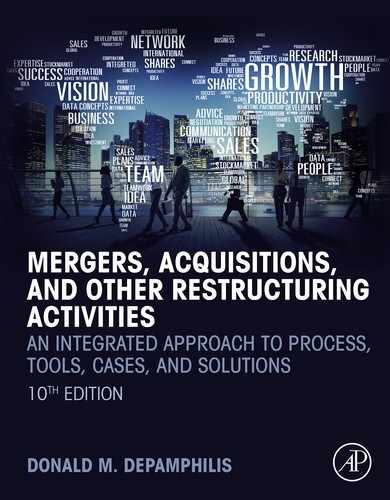
The initial offer price for Target lies between the minimum19and maximum offer prices. In a stock purchase deal,20 the minimum price is Target’s stand-alone present value (PVT) or its current market value (MVT) (i.e., Target’s current stock price times its shares outstanding). The maximum price is the sum of the minimum price plus the PV of net synergy (PVNS).21 The initial offer price (PVIOP) is the sum of the minimum purchase price and a percentage, α between 0 and 1, of PVNS. Exhibit 14.4 provides an algebraic illustration of how the initial offer price is determined and a numerical example of how the offer price premium and multiple can be determined for a given offer price.
Exhibit 14.4
Determining the Offer Price (PVOP)—Purchase of Stock
- a. PVMIN = PVT or MVT, whichever is greater. MVT is Target’s current share price times the number of shares outstanding
- b. PVMAX = PVMIN + PVNS, where PVNS = PV (sources of value) − PV (destroyers of value)
- c. PVOP = PVMIN + α PVNS, where 0 ≤ α ≤ 1
- d. Offer price range for Target = (PVT or MVT) < PVOP < (PVT or MVT) + PVNS
Once the dollar value of the offer price has been determined, the offer price per share, premium and offer (purchase) price multiple can be determined as follows:
Assumptions:
- Target’s predeal price per share = $18
- Target shares outstanding = 5 million
- Target’s current earnings per share = $2.20
- Target’s minimum (standalone or market) value = $100 million
- PV of net synergy = $20 million
- Alpha (α) = 50%
Solution:
- Offer (purchase) price premium = $22/$18 = 22.2%
- Offer (purchase) price multiple = $22/$2.20 = 10a
Note α represents that portion of net synergy shared with target shareholders and not the purchase price premium. Once the offer price has been determined, the purchase price premium may be estimated by comparing the offer price to Target’s preannouncement share price. The offer price should be compared to similar deals to determine if it is excessive.22
To determine α, Acquirer may estimate the portion of net synergy supplied by Target. Cash flows due to synergy are those that arise only because of the combination of the firms. The percentage of net synergy contributed by Target can be estimated by calculating the contribution to incremental operating profit attributable to cross-selling or to cost savings resulting from a reduction in the number of Target employees or elimination of other Target related overhead such as leased facilities. Additional Target-related synergy could include intellectual property whose value is represented by the potential profit generated by selling such property to others or from new products based on Target copyrights or patents. Ultimately, what fraction of synergy is negotiated successfully by Target depends on its leverage or influence relative to Acquirer.23
If it is determined that Target would contribute 30% of net synergy, Acquirer may share up to that amount with Target’s shareholders. Acquirer may share less than 30% if it is concerned that realizing synergy on a timely basis is problematic. To discourage potential bidders, Acquirer might make a preemptive bid so attractive that Target’s board could not reject the offer for fear of possible shareholder lawsuits, resulting in more than 30% of net synergy shared with Target. How high to make the preemptive bid can be influenced by security analysts’ projected share prices for a firm. Target’s shareholders may use security analyst price projections for Target as reference points such that the higher the initial offer price is relative to the reference point the greater the likelihood the deal will be completed.24
The offer price should fall between the minimum and maximum prices for three reasons. First, it is unlikely that Target can be purchased at the minimum price, because Acquirer normally has to pay a premium to induce Target’s shareholders to sell their shares. In an asset purchase, the rational seller would not sell at a price below the after-tax liquidation value of acquired assets less assumed liabilities, since this represents what the seller could obtain by liquidating rather than selling the assets. Second, at the maximum end of the range, Acquirer would be ceding all of the net synergy created by combining the two firms to Target’s shareholders. Finally, it often is prudent to pay significantly less than the maximum price, because of the uncertainty of realizing estimated synergy on a timely basis.
Step 4 (b) Compare Projected Credit Ratios With Industry Average Ratios
Table 14.11 shows the impact of increased borrowing on Newco’s projected credit ratios in comparison to current industry averages. Investors often use such comparisons to assess a firm’s solvency and liquidity. This table measures the magnitude of Newco’s projected debt burden (debt-to-total capital ratio) and ability to repay its debt (interest coverage ratio).25 The higher the debt-to-total capital ratio relative to the industry average the more investors will become concerned about the potential insolvency of the firm (i.e., the likelihood the firm will be unable to pay its outstanding debt if liquidated). Similarly, investors could view the liquidity of a firm with a low interest coverage ratio compared to the industry as problematic.

Assume that the current industry average credit ratios will prevail during the forecast period. Does Newco’s projected debt-to-total capital ratio exceed significantly the average for the industry? Does the firm’s projected interest coverage fall substantially below the industry average due to the increase in the firm’s indebtedness? Will Newco not be in compliance with pretransaction loan covenants? Is the firm’s credit rating in jeopardy? If the answer to these questions is yes, it may be impractical to finance the deal under the proposed capital structure.
One method for determining an appropriate financing or postclosing capital structure is to establish a target credit rating for Newco.26 Firms often desire at least an investment grade rating (for firms exhibiting a relatively low risk of default) to limit an increase in borrowing costs. Achieving a specific credit rating requires the firm to achieve certain credit ratios, measured as debt-to-total capital and interest coverage ratios. The magnitude of these ratios will be affected by the size of the firm and the industry in which it competes. Larger firms are expected to be better able to repay their debts in liquidation due to their greater asset value. Firms with stable cash flows are considered less risky than those whose cash flows are cyclical and therefore less predictable. Deviating from a target capital structure can result in fluctuations in institutional ownership and in turn the firm’s share price.27
Step 4 (c) Determine Impact of Deal on Newco EPS
Newco’s EPS will be impacted by Acquirer’s and Target’s projected earnings plus the contribution to future earnings from net synergy. EPS will also be affected by the number of Acquirer shares exchanged for each Target share plus any Acquirer shares issued to raise cash to finance the cash portion of the purchase price. In addition to credit ratios, Table 14.11 also displays Newco’s projected EPS and how this compares to what Acquirer would have earned per share had it not completed the deal. Despite the issuance of a large number of Acquirer shares to complete the deal, Newco EPS and cash flow per share are sharply higher following completion of the deal than they would have been had the transaction not been undertaken.
Acquirers often adjust or normalize earnings per share during the first full year in which they operate Target for that portion of transaction-related expenses that cannot be amortized and for integration expenditures. Consistent with GAAP, such expenses would be deducted from consolidated earnings before determining EPS and reporting such figures to the Securities and Exchange Commission. However, so-called adjusted EPS is calculated by adding to GAAP-based EPS transaction and integration expenses per share to show what the consolidated performance would be without these nonrecurring expenses.
To calculate Newco’s postclosing EPS, estimate the number of new Acquirer shares issued to complete the deal. The exchange of Acquirer’s shares for Target’s shares requires the calculation of the appropriate share-exchange ratio (SER). The SER can be negotiated as a fixed number of shares of Acquirer’s stock to be exchanged for each share of Target’s stock. Alternatively, SER can be defined in terms of the dollar value of the negotiated offer price per share of Target stock (POP) to the dollar value of Acquirer’s share price (PA). The SER is calculated by the following equation:
The SER can be less than, equal to, or greater than 1, depending on the value of Acquirer’s shares relative to the offer price on the date set during the negotiation for valuing the transaction. Exhibit 14.5 illustrates how share exchange ratios are used to estimate the number of Acquirer shares that must be issued in a share for share exchange and the resulting ownership distribution between Acquirer and former Target shareholders.
The number of new Acquirer shares issued to complete a deal also is affected by such derivative securities as options issued to Target’s employees and warrants, as well as convertible securities. Such securities derive their value from the firm’s common stock into which they may be converted. Upon conversion, these securities result in additional common shares that must be purchased by a buyer wishing to avoid minority shareholders following a takeover. Such securities are commonly assumed to have been converted in calculating fully diluted shares outstanding, that is, the number of Target’s “basic” shares outstanding (i.e., pretransaction shares outstanding) plus the number of shares represented by the firm’s “in the money” options, warrants, and convertible debt and preferred securities. Basic shares are found are found on the cover of a firm’s most recent 10Q or 10K submission to the SEC. Options and convertible securities information are found in the firm’s most recent 10K.
Granted to employees, stock options represent noncash compensation and offer the holder the right to buy (call) shares of the firm’s common equity at a predetermined “exercise” price.28 Option holders are said to be vested once the required holding or “vesting” period expires, and their options can be converted into shares of the firm’s common equity. An option is considered to be “in the money” whenever the firm’s common share price exceeds the option’s exercise price; otherwise, they are “out of the money.” Warrants are securities often issued along with debt and entitle holders of the debt to buy the firm’s common shares at a preset price during a given time period. It is common to assume that only “in-the-money” options and warrants will be converted as a result of a takeover. However, all options and warrants can be exercised, regardless of their vesting status (i.e., vested or not vested) and exercise price, in the event of a hostile takeover if they include change of control provisions.29
The treasury method assumes all in the money options and warrants, since they are issued at different times and prices, are exercised at their weighted average exercise price30 and option proceeds are assumed used to repurchase outstanding Target shares at the company’s current share price. Since the exercise price is less than the current price of target shares (which has risen to approximately the level of the offer price), the dollar proceeds received by the firm when holders exercise their options and warrants enable the firm to repurchase fewer shares than had been exercised. Therefore, the number of shares outstanding will increase by the difference between the number of options exercised and those repurchased.31
In Table 14.12, 4.045 options, whose weighted average exercise price is $37.46, are assumed to be converted as they are well below the offer price of $82 per Target share. The net increase in the value of shares outstanding resulting from the exercise of options equals the dollar value of such shares valued at the firm’s current share price less the value of option proceeds expressed at the weighted average exercise price of $180.16 million [i.e., ($82 − $37.46) × 4.045]. This figure represents the value of shares the firm is unable to repurchase with the proceeds received from exercised options. Therefore, the net increase in shares outstanding resulting from the exercising of options equals 2.1971 (i.e., $180.16/$82).32

The same table also illustrates how other types of convertible securities must be considered when calculating the number of target shares to be acquired. If convertible securities are present, it is necessary to add to Target’s basic shares outstanding the number of new shares issued following the conversion of such securities. Convertible securities include preferred stock and debt. Information on the number of options outstanding, vesting periods, and their associated exercise prices, as well as convertible securities, are available in the footnotes to Target’s financial statements. It is reasonable to assume that such securities will be converted to common equity when the conversion price is less than the offer price per share.
Convertible preferred stock can be exchanged for common stock at a specific price at the discretion of the shareholder. The value of the common stock for which the preferred stock is exchanged is called the conversion price. If the preferred stock is convertible into 1.75 common shares and is issued at a par value of $100, the price at which it can be converted (i.e., its conversion price) is $57.14 (i.e., $100/1.75). That is, the preferred shareholder would receive 1.75 shares of common stock if the preferred shareholder choses to convert when the common share price exceeds $57.14. Similarly, convertible debt can be converted into a specific number of common shares and is normally denominated in units of $1000. If when issued buyers of such debt were given the right to convert each $1000 of debt they held into 20 common shares, the implied conversion price would be $50 (i.e., $1000/20).
Table 14.12 also illustrates the additional common shares created due to the conversion of in-the-money options and warrants as well as convertible preferred stock and debt. Following conversion, the total number of new shares into common shares that must be added to the number of basic target shares is 2.2654 million shares (i.e., 2.1971 + 0.0088 + 0.0595). This will add $185.75 million (i.e., 2.2653 × $82) to the purchase price for 100% of Target’s shares.
Unless addressed in the preclosing negotiation, executive stock options subject to early exercise such as in a takeover can result in a larger valuation discount from their true value than if exercised voluntarily. Why? Target firm executives forfeit more of the option’s time value than might have been the case if voluntarily exercised. Most option valuation methodologies are based on voluntary valuation.33
Step 4 (d) Determine If the Deal Will Allow Newco to Meet or Exceed Required Returns
Newco’s minimum required financial return is its weighted average cost of capital (WACC). Standard capital budgeting theory tells us that a firm will meet or exceed its cost of capital as long as the net present value (NPV) of a discrete investment is greater than or equal to zero. Acquirer’s investment in Target is not only the equity consideration (EQC), but also any transaction expenses (TE) associated with closing the deal. Equity consideration refers to what Acquirer pays for Target’s equity. Therefore, the challenge for Acquirer is to create sufficient value by combining the two firms such that the following is true:
PVTarget and PVNetSynergy are the present values of Target as a standalone business and the net synergy resulting from combining Target and Acquirer.
The valuation section of Acquirer Transaction Summary Worksheet (Table 14.3) indicates that about $7.4 billion in incremental value or net synergy is created by Acquirer’s takeover of Target. This implies that the financial return on the purchase of Target is well in excess of Acquirer’s WACC or minimum required rate of return on assets.
Depending upon size and deal complexity, as well as how they are financed, transaction expenses approximate 3%–5% of the purchase price, with this percentage decreasing for larger deals. To estimate such expenses, distinguish between financing-related and nonfinancing related expenses. Financing related expenses for M&As can equal 1%–2% of the dollar value of bank debt and include fees for arranging the loan and for establishing a line of credit. Fees for underwriting nonbank debt can average 2%–3% of the value of the debt. Nonfinancing related fees often represent as much as 2% of the purchase price and include investment banking, legal, accounting, and other consulting fees. For accounting purposes, nonfinancing-related expenses are expensed in the year in which the deal closes, while those related to deal financing are capitalized on the balance sheet and amortized over the life of the loan.
M&A Models: Asset Purchases
As with a stock purchase model, asset purchases begin with the estimation of Target’s enterprise value. Viewed in this context as total Target assets (TA), the enterprise value is then adjusted by subtracting Target assets excluded from the deal (Aexcl)34 and Target liabilities included in the deal (Linc), that is, assumed by the buyer.35 The end result is referred to as net acquired assets.36
Aincl equals Target assets included in the deal (i.e., assumed by the buyer). The purchase price is what Acquirer pays for net acquired assets and is expressed as a multiple of net book assets. This multiple should be compared to recent comparable deals to determine its reasonableness. The purchase price should lie between the minimum (i.e., after-tax liquidation value of the assets less liabilities) and the maximum price (i.e., minimum price plus net synergy).
It is common for buyers to purchase selected assets and to assume responsibility for short-term seller operating liabilities. Such liabilities include payables and such items as accrued vacation, employee benefits, bonuses, commissions, etc., to ensure a smoother transition for those Target employees transferring to Acquirer. Acquirer may also assume responsibility for other liabilities such as product warranty claims that have not been satisfied to ensure that they are paid in order to retain customer loyalty.
Assume that Acquirer pays $90 million to purchase $75 million in net acquired assets, consisting of $100 million of Target net property, plant and equipment (i.e., Net PP&E) less assumed Target current liabilities of $25 million and that the book values of Target assets and liabilities are equal to their fair market value.37 The implied purchase price multiple is 1.2 times net acquired assets (i.e., $90 million/$75 million), a 20% premium.
Sales, cost of sales, and operating income associated with the net acquired assets, as well as any additional interest expense incurred to finance the purchase and expenses incurred to integrate the acquired assets, are added to Acquirer’s income statement (Table 14.13). For this illustration, the adjustments’ column shows the addition of Target’s sales, cost of sales, additional interest expense, and taxes to Acquirer’s income statement. Incremental revenue generated by selling Acquirer products to Target’s customers is assumed to be $200 million. Target’s cost of sales before the deal was $195 million, which is reduced by anticipated cost-related synergy of $5 million. Expenditures related to integrating Target assets are $15 million. A one-time $10 million noncash gain is added to Acquirer’s income statement, because it is buying Target’s assets at a discount from their book value (i.e., paying $90 million for $100 million in Net PP&E). Acquirer is able to negotiate the favorable purchase of Net PP&E because of its willingness to assume certain Target liabilities. Incremental interest expense related to financing the deal is $7 million. Taxes paid for purposes of illustration are calculated at the firm’s assumed marginal tax rate of 40%. The addition of the assets is expected to increase Acquirer’s net income in subsequent years due to anticipated cost savings as a result of productivity improvements and incremental revenue from cross-selling former Target products to Acquirer’s customers.
Table 14.13
| Acquirer predeal | Adjustments | Acquirer postdeal | |
|---|---|---|---|
| Sales | $1750.0 | $200.0 | $1950.0 |
| Cost of sales | 1488.0 | 190.0 | 1678.0 |
| Integration expense | 15.0 | 15.0 | |
| EBIT | 262.0 | 257.0 | |
| Other income | 0.0 | 10.0 | 10.0 |
| Net interest expense | 30.0 | 7.0 | 37.0 |
| EBT | 232.0 | 230.0 | |
| Tax @ 0.40 | 92.8 | (0.8) | 92.0 |
| Net income | $139.2 | $138.0 |

In consolidation, the dollar value of net acquired assets is recorded on Acquirer’s balance sheet by adding the purchased assets to Acquirer’s assets and assumed liabilities to Acquirer’s liabilities. In addition, entries are made to the liability/equity side of Acquirer’s balance sheet to show how the purchase is to be financed. Table 14.14 illustrates Acquirer’s balance sheet adjustments made to reflect the purchase of specific Target assets and the assumption of certain Target liabilities. Goodwill (i.e., the difference between the purchase price and the fair market value of net acquired assets) equals $15 million (i.e., $90 million less $75 million). The purchase is financed by using $20 million in Acquirer pretransaction cash balances and by borrowing $70 million in long-term debt at a 10% interest rate. Consequently, the entries in the adjustments column include a $20 million reduction in cash and an increase of $100 million in Net PP&E, $15 million in goodwill, $25 million for assumed current liabilities, and $70 million in new debt.

Table 14.15 shows the cash flow statement for the purchase of the previously described net acquired assets. Ending cash balances in 2015 are reduced by $20 million to partially finance the purchase of the $100 million in Target Net PP&E. Acquirer net income of ($1.2) million represents the difference between predeal net income of $139.2 and postdeal net income of $138.0 million. Negative net income during the first full year of operation including the net acquired assets resulted from integration expenses and incremental interest expense exceeding the positive contribution of operating income and the one-time gain. The one-time gain of $10 million due to the purchase of Net PP&E at a discount is eliminated in the calculation of cash flow, because it does not involve the actual receipt of cash. Current liabilities increase cash flow from operations by the amount of assumed Target liabilities. Cash flow from investing activities decreases by the amount paid for Net PP&E while cash flow from financing activities increases by what is borrowed.

Quantifying Synergy
Acquirers sometimes overpay because they overestimate synergy. Substantial effort should be given to estimate accurately the incremental value that can be realized by combining firms. Models can be simulated to estimate a range of postmerger synergies using premerger product prices and production costs. Such models provide estimates of overall efficiency improvements and combined firms’ pricing power.38 When there is uncertainty associated with quantifying potential synergy due to limited reliable information, acquirers tend to assign a lower value to the target firm to increase the potential for acquirer shareholder value creation.39 There are three general categories of synergy: revenue-related, cost-related, and operating/asset-related synergy.40 These are discussed next.
Revenue-Related Synergy
The customer base for the target and acquiring firms can be segmented into three categories: (1) those served only by the target, (2) those served only by the acquirer, and (3) those served by both firms. The first two segments may represent revenue enhancement opportunities by enabling the target or the acquirer to sell its current products into the other’s current customer base. The third segment could represent a net increase or decrease in revenue for the new firm. Incremental revenue may result from new products that could be offered only as a result of exploiting the capabilities of the target and acquiring firms in combination. However, revenue may be lost as some customers choose to have more than one source of supply. The analysis of incremental revenue opportunities is simplified by focusing on the largest customers, because it often is true that 80% of a company’s revenue come from about 20% of its customers. Incremental revenue can be estimated by having the sales force provide estimates of the potential additional revenue that could be achieved from having access to new customers and offering current customers new products. In general, such revenue can be realized over time as the target’s and acquirer’s sales forces must be trained to sell each other’s products.
Target firms with strong customer relationships often receive higher merger premiums than those that don’t as acquirers often assume they can retain those accounts.41 Consequently, acquirers often overpay. Later they discover they are unable to retain those customer accounts resulting in a significant loss of revenue through customer attrition. Paying a premium for strong customer relationships may only make sense when the target has long-term, profitable contracts in place with its largest customers.
Cost Savings-Related Synergies
The cost of sales for the combined firms may be adjusted for cost savings resulting from such factors as the elimination of redundant jobs. Cost savings tend to be greatest between firms with overlapping employees with similar skills (so-called “human capital relatedness”) as the acquiring firm often is able to negotiate lower wage and benefit packages with target firm employees and has the option of retaining only the most productive employees.42
Direct labor refers to those employees directly involved in the production of goods and services. Indirect labor refers to supervisory overhead and administrative support staff. A distinction needs to be made because of likely differences in average compensation for direct and indirect labor. Sales, general, and administrative expenses (S,G,&A) may be reduced by the elimination of overlapping jobs and the closure of unneeded sales offices resulting in lease expense savings. However, leased space may be eliminated prior to the lease expiration date by paying off the balance of what is owed. For an illustration of how to quantify revenue-related synergy; gross margin improvement; and sales, general and administrative synergy, see Table 14.16. The projected data for incremental sales, gross margin improvement, and SG&A savings serve as inputs into the synergy section of the Summary Worksheet of the model. Headcount figures shown in 2018 are held constant in subsequent years reflecting that the savings continue indefinitely or until terminated employees are replaced.
Table 14.16
| 2016 | 2017 | 2018 | 2019 | 2020 | ||||
|---|---|---|---|---|---|---|---|---|
| ($millions) | ||||||||
| Revenue-related synergy | ||||||||
| New customers for Acquirer products | 15,000,000 | 30,000,000 | 50,000,000 | 50,000,000 | 50,000,000 | |||
| New customers for Target products | 20,000,000 | 25,000,000 | 40,000,000 | 40,000,000 | 40,000,000 | |||
| New product revenue | 0 | 25,000,000 | 60,000,000 | 60,000,000 | 60,000,000 | |||
| Loss from customer attrition | − 10,000,000 | − 5,000,000 | 0 | 0 | 0 | |||
| Total incremental sales | 25,000,000 | 75,000,000 | 150,000,000 | 150,000,000 | 150,000,000 | |||
| Gross margin improvement | ||||||||
| Cost of sales | ||||||||
| Headcount reduction—direct labor | 40 | 77 | 109 | 109 | 109 | |||
| Average salary and benefits | 69,000 | 69,515 | 69,910 | 69,910 | 69,910 | |||
| Direct labor savings | 2,760,000 | 5,352,655 | 7,620,190 | 7,620,190 | 7,620,190 | |||
| Headcount reduction—indirect labor | 28 | 57 | 90 | 90 | 90 | |||
| Average salary and benefits | 80,000 | 81,535 | 82,000 | 82,000 | 82,000 | |||
| Indirect labor savings | 2,240,000 | 4,647,495 | 7,380,000 | 7,380,000 | 7,380,000 | |||
| Total direct and indirect labor savings | 5,000,000 | 10,000,150 | 15,000,190 | 15,000,190 | 15,000,190 | |||
| Sales, general and administrative savings | ||||||||
| Headcount reduction —direct sales | 16 | 21 | 38 | 38 | 38 | |||
| Average salary and benefits | 90,000 | 91,500 | 92,000 | 92,000 | 92,000 | |||
| Selling expense savings | 1,440,000 | 1,921,500 | 3,496,000 | 3,496,000 | 3,496,000 | |||
| Headcount reduction —administrative | 20 | 36 | 52 | 52 | 52 | |||
| Average salary and benefits | 78,000 | 79,000 | 80,000 | 80,000 | 80,000 | |||
| General and administrative savings | 1,560,000 | 2,844,000 | 4,160,000 | 4,160,000 | 4,160,000 | |||
| Total SG&A savings | 3,000,000 | 4,765,500 | 7,656,000 | 7,656,000 | 7,656,000 | |||
| Leased space savings (net of buyout) | 0 | 234,500 | 344,000 | 344,000 | 344,000 | |||
| Total SG&A savings | 3,000,000 | 5,000,000 | 8,000,000 | 8,000,000 | 8,000,000 | |||

Operating/Asset-Related Synergies
Additional cash can be generated by better managing the combined firms’ net operating assets, both fixed assets and working capital. With respect to fixed assets such as plant and equipment, production can be centralized in a single facility to take advantage of economies of scale as the facility may be utilized more fully. Economies of scope can be realized by having a single department (e.g., human resources and accounting) support multiple product lines or by combining regional sales offices. The combined firms may be able to reduce the amount of money tied up in working capital by deferring payment of bills and shortening the time required to convert products into cash. The time it takes to convert inventory to cash is the average length of time in days required to produce and sell finished goods. The receivables collection period is the average length of time in days required to collect receivables. The payables deferral period is the average length of time in days between the purchase of and payment for materials and labor. By reducing this time it takes to generate cash and deferring payables, without affecting the operating profit margin or sales, profits and cash flow increase and in turn firm value.43
Things to Remember
M&A modeling facilitates deal valuation, structuring, and financing. Acquirers may use models to estimate the value of Target before making a formal bid and the appropriate capital structure to finance the deal. Targets use models to estimate the value of the combined businesses and their contribution to synergy. Both acquirers and targets use models to review the implications of proposals and counterproposals that arise before an agreement is reached.
Chapter Discussion Questions
- 14.1 Why should a target company be valued as a stand-alone business? Give examples of the types of adjustments that might have to be made if Target is part of a larger company.
- 14.2 Why should “in the money” options, warrants, and convertible preferred stock and debt be included in the calculation of the purchase price to be paid for Target?
- 14.3 What are value drivers? How can they be misused in M&A models?
- 14.4 Can the offer price ever exceed the maximum purchase price? If yes, why? If no, why not?
- 14.5 Why is it important to clearly state assumptions underlying a valuation?
- 14.6 Assume two firms have little geographic overlap in terms of sales and facilities. If they were to merge, how might this affect the potential for synergy?
- 14.7 Dow Chemical, a leading manufacturer of chemicals, in announcing that it had an agreement to acquire competitor Rohm and Haas, said it expected to broaden its current product offering by offering the higher-margin Rohm and Haas products. What would you identify as possible synergies between these two businesses? In what ways could the combination of these two firms erode combined cash flows?
- 14.8 Dow Chemical’s acquisition of Rohm and Haas included a 74% premium over the firm’s preannouncement share price. What is the possible process Dow employed in determining the stunning magnitude of this premium?
- 14.9 For most transactions, the full impact of net synergy will not be realized for many months. Why? What factors could account for the delay?
- 14.10 How does the presence of management options and convertible securities affect the calculation of the offer price for Target?
Answers to these Chapter Discussion Questions are available in the Online Instructor’s Manual for instructors using this book (https://textbooks.elsevier.com/web/Manuals.aspx?isbn=9780128150757).
Practice Problems and Answers
- 14.11 Acquiring Company is considering the acquisition of Target Company in a share-for-share transaction in which Target Company would receive $50.00 for each share of its common stock. Acquiring Company does not expect any change in its P/E multiple after the merger.
Acquiring Co. Target Co. Earnings available for common stock $150,000 $30,000 Number of shares of common stock outstanding 60,000 20,000 Market price per share $60.00 $40.00 Using the preceding information about these two firms and showing your work, calculate the following:
- a. Purchase price premium. Answer: 25%
- b. Share-exchange ratio. Answer: 0.8333
- c. New shares issued by Acquiring Company. Answer: 16,666
- d. Total shares outstanding of the combined companies. Answer: 76,666
- e. Postmerger EPS of the combined companies. Answer: $2.35
- f. Premerger EPS of Acquiring Company. Answer: $2.50
- g. Postmerger share price. Answer: $56.40, compared with $60.00 premerger
- h. Postmerger ownership distribution. Answer: Target shareholders = 21.7% and Acquirer shareholders = 78.3%
- 14.12 Acquiring Company is considering buying Target Company. Target Company is a small biotechnology firm that develops products licensed to the major pharmaceutical firms. Development costs are expected to generate negative cash flows during the first 2 years of the forecast period of $(10) million and $(5) million, respectively. Licensing fees are expected to generate positive cash flows during years 3–5 of the forecast period of $5 million, $10 million, and $15 million, respectively. Because of the emergence of competitive products, cash flow is expected to grow at a modest 5% annually after the fifth year. The discount rate for the first 5 years is estimated to be 20% and then drop to the industry average rate of 10% beyond the fifth year. Also, the present value of the estimated net synergy created by combining Acquiring and Target companies is $30 million. Calculate the minimum and maximum purchase prices for Target Company. Show your work.
Answer: Minimum price: $128.5 million; Maximum price: $158.5 million. - 14.13 Using the information given below, calculate fully diluted shares. Assume the firm uses proceeds received from the conversion of options to common shares to repurchase as many of these new shares as possible. Select the correct answer from (a) to (e).
Calculating fully diluted shares outstanding $million, except per share data, shares in millions Current share price $30.00 Basic shares outstanding 200.00 Options that can be exercised 40.0 Weighted average exercise price $20.00 
- a. 224.52
- b. 263.59
- c. 213.33
- d. 256.87
- e. 233.47
Answer: C
- 14.14 What is the fully diluted offer price (equity value) for a tender offer made to acquire a target whose pretender shares are trading for $1.50 per share? The tender offer includes a 30% premium to the target’s pretender share price. The target has basic shares outstanding of 70 million and 5 million options which may be converted into common shares at $1.60 per share.
Answer: $138.25 million - 14.15 Using the M&A Valuation and Deal Structuring Model on the website accompanying this text (see the website address in the Chapter Overview section at the beginning of this chapter) and the data contained in the cells as a starting point, complete the following:
- a. What is the enterprise and equity value of Target on the Valuation Worksheet?
- b. Increase the sales growth rate by one percentage point (i.e., to 6.5%) on the Target Assumptions Worksheet. What is the impact on the Target’s enterprise and equity values? (Hint: See Valuation Worksheet.) Undo change or close model but do not save results in order to restore the model’s original data.
Answers: - a. Before change to revenue growth assumption by one percentage point:
- 1. Target enterprise value: $11,582.2
- 2. Target equity value: $9796.8
- b. After change in revenue growth assumption by one percentage point
- 1. Target enterprise value: $12,356.3
- 2. Target equity value: $10,570.9
- 14.16 Using the M&A Valuation and Deal Structuring Model accompanying this text (see the website address in the “Chapter Overview” section at the beginning of this chapter) and the data contained in the cells as a starting point, complete the following:
- a. What is the enterprise and equity value of Target on the Valuation Worksheet?
- b. On the worksheet named Target Assumptions, increase COGS (cost of goods sold) as a percent of sales by one percentage point (i.e., 0.43–0.44) on the Target Assumptions Worksheet. What is the impact on the Target’s enterprise and equity values? (Hint: See Valuation Worksheet.) Undo change or close the model but do not save the results in order to restore the model’s original data.
Answers: - a. Before change to COGS ratio by one percentage point:
- 1. Target enterprise value: $11,582.2
- 2. Target equity value: $9796.8
- b. After change in COGS ratio by one percentage point:
- 1. Target enterprise value: $11,104.8
- 2. Target equity value: $9319.4
- 14.17 Using the M&A Valuation and Deal Structuring Model accompanying this text (see the website address in the “Chapter Overview” section at the beginning of this chapter):
- a. On the Valuation Worksheet, note the enterprise and equity values for Newco.
- b. On the Summary worksheet under Incremental Sales Synergy, change incremental revenue to $200 million in the first year, $250 million in the second year, and $350 in the third year. What is the impact on Newco’s enterprise and equity values? (Hint: See Valuation Worksheet.) Undo changes or close the model but do not save the results.
Answers: - a. Before incremental sales growth:
- 1. Newco enterprise value: $32,813.7
- 2. Newco equity value: $20,970.8
- b. After change in incremental sales:
- 1. Newco enterprise value: $33,766.5
- 2. Newco equity value: $21,923.6
- 14.18 Using the M&A Valuation and Deal Structuring Model accompanying this text (see the website address in the “Chapter Overview” section of this chapter):
- a. On the Transaction Summary Worksheet, under the heading Form of Payment, change the composition of the purchase price to 100% cash. Assume the purchase price is partially financed by reducing Acquirer excess cash by $1 billion and by raising $4 billion by issuing new Acquirer equity. Under the Sources and Uses heading, how is the remainder of the purchase price financed?
- b. Change the composition of the purchase price to 100% equity, what is the impact on how the purchase price is financed? Close model but do not save the results.
Answers: - a. Form of Payment = 100% cash. Senior debt is increased by $10,129.8 million.
- b. Form of Payment = 100% equity. Senior debt shows a negative $4365 million, which does not make sense. Set excess cash and new common shares issued to public equal to zero. Senior Debt automatically increases by $635 million.
Solutions to these Practice Problems are available in the Online Instructor’s Manual for instructors using this book (https://textbooks.elsevier.com/web/Manuals.aspx?isbn=9780128150757).
Almost 9 months after reaching an agreement to combine their operations, the merger between Life Technologies Corporation (Life Tech) and Thermo Fisher Scientific Inc. (Thermo Fisher) was completed on January 14, 2014. Thermo Fisher is the largest provider by market value of analytical instruments, equipment, reagents and consumables, software, and services for scientific research, analysis, discovery, and diagnostics applications. Life Tech is the second largest by market value provider of similar products and services to the scientific research and genetics analysis communities. Life Tech had been evaluating strategic options for the firm since mid-2012, concluding that putting itself up for sale would be the best way to maximize shareholder value (see the Case Study at the end of Chapter 11 for more detail). This case study utilizes the publicly announced terms of the merger of Life Tech into a wholly owned subsidiary of Thermo Fisher, with Life Tech surviving. The terms were used to develop pro forma financial statements for the combined firms. These statements are viewed as a “base case.”44
The financial model discussed in this chapter is used to show how changes in key deal terms and financing structures impacted the base case scenario. The discussion questions following the case address how the maximum offer price for Life Tech could be determined, what the impact of an all-debt or all-equity deal would have on the combined firms’ financial statements, and the implications of failing to achieve synergy targets. Such scenarios represent the limits of the range within which the appropriate capital structure could fall and could have been part of Thermo Fisher’s predeal evaluation. As announced by Thermo Fisher, the appropriate capital structure is that which maintains an investment grade credit rating following the merger. Thermo Fisher’s senior management could have tested various capital structures between the two extremes of all-debt and all-equity before reaching agreement on the form of payment with which they were most comfortable. Therefore, the form of payment and how the deal was financed were instrumental to the deal getting done.
According to the terms of the deal, Thermo Fisher acquired all of Life Tech’s common shares, including all vested and unvested outstanding stock options, at a price of $76 per share in cash, with the Life Tech shares canceled at closing. The actual purchase price consisted of an equity consideration of $13.6 billion plus the assumption of $2.2 billion of Life Tech’s outstanding debt. The purchase price was funded by a combination of new debt, equity, and cash on Thermo Fisher’s balance sheet. Thermo Fisher executed a commitment letter, dated April 14, 2013, with JPMorgan Chase Bank, N.A., J.P. Morgan Securities LLC and Barclays Bank PLC that provided a commitment for a $12.5 billion 364-day unsecured bridge loan facility. The facility enabled the firm to pay for much of the purchase price before arranging permanent financing by issuing new debt and equity in late 2013.
In an effort to retain an investment grade credit rating45 by limiting the amount of new borrowing, Thermo Fisher issued new common equity and equity linked securities such as convertible debt and convertible preferred totaling $3.25 billion to finance about one-fourth of the $13.6 billion equity consideration. The $3.25 billion consisted of $2.2 billion of common stock sold in connection with its public offering prior to closing, and up to a maximum of $1.05 billion of additional equity to be issued at a later date in the form of convertible debt and preferred shares. Thermo Fisher financed the remaining $10.35 billion of the purchase price with the proceeds of subsequent borrowings and $1 billion in cash on its balance sheet.
Thermo Fisher and Life Tech compete in the medical laboratory and research industry. The average debt-to-total capital ratio for firms in this industry is 44.6%,46 and the average interest coverage ratio is 4.0.47 Thermo Fisher expects that available free cash flow will allow for a rapid reduction in its debt. The firm expects to be below the industry average debt-to-total capital ratio by the end of the third full year following closing and about 12 percentage points below it within 5 years after closing. The firm’s interest coverage ratio is expected to be equal to the industry average by the second year and well above it by the third year and beyond. These publicly stated goals established metrics shareholders and analysts could use to track the Thermo Fisher’s progress in integrating Life Tech.
Consistent with management’s commitment to only make deals that immediately increase earnings per share, Thermo Fisher expects the deal to increase adjusted earnings per share during the first full year of operation by as much as $0.70–$1.00 per share. Adjusted earnings per share exclude the impact on earnings of transaction-related expenses and expenses incurred in integrating the two businesses. Including these expenses in the calculation of EPS is expected to result in a $(0.16) per share during the first full year following closing, but excluding these expenses will result in $0.99 per share.48
Realizing synergy on a timely basis would be critical for Thermo Fisher to realize its publicly announced goal that the deal would be accretive on an adjusted earnings per share basis at the end of the first full year of operation. Synergies anticipated by Thermo Fisher include the realization of additional gross margin of $75 million and the realization of $20 million in SG&A savings in 2014, the first full year following closing. Gross margin improvement and SG&A savings are projected to grow to $225 million and $100 million, respectively, by 2016, and to be sustained at these levels indefinitely. Most of the cost savings are expected to come from combining global infrastructure operations. Revenue-related synergy is expected to reach $300 million annually from cross-selling by the third year, up from $25 million in the first year.
Mark Fisher, CEO of Thermo Fisher knew that the key to unlocking value for shareholders once the deal closed was realizing the anticipated synergy on a timely basis. However, rationalizing facilities by reducing redundant staff, improving gross margins and increasing revenue was fraught with risk. Eliminating staff had to be done in such a way as not to demoralize employees and increasing revenue could only be achieved if the loss of existing customers due to the attrition that often follows M&As could be kept to a minimum. Having been through postmerger integrations before, he knew first-hand the challenges accompanying these types of activities. At the time of closing, many questions remained. What if synergy were not realized as quickly and in the amount expected? What if expenses and capital outlays would be required in excess of what had been anticipated? How patient would shareholders be if the projected impact on earnings per share was not realized? Only time would tell.
Discussion Questions
Answer questions 1–4 using as the base case the firm valuation and deal structure data in the Microsoft Excel model available on the companion site to this book entitled Thermo Fisher Acquires Life Technologies Financial Model. Please see the “Chapter Overview” section of this chapter for the site’s internet address. Assume that the base case assumptions were those used by Thermo Fisher in its merger with Life Tech. The base case reflects the input data described in this case study. To answer each question you must change selected input data in the base case, which will change significantly the base case projections. After answering a specific question, either undo the changes made or close the model and do not save the model results. This will cause the model to revert back to the base case. In this way, it will be possible to analyze each question in terms of how it is different from the base case.
- 1. Thermo Fisher paid $76 per share for each outstanding share of Life Tech. What is the maximum offer price Thermo Fisher could have made without ceding all of the synergy value to Life Tech shareholders? (Hint: Using the Transaction Summary Worksheet, increase the offer price until the NPV in the section entitled Valuation turns negative.) Why does the offer price at which NPV turns negative represent the maximum offer price for Life Tech? Undo changes to the model before answering subsequent questions.
- 2. Thermo Fisher designed a capital structure for financing the deal that would retain its investment grade credit rating. To do so, it targeted a debt-to-total capital and interest coverage ratio consistent with the industry average for these credit ratios. What is the potential impact on Thermo Fisher’s ability to retain an investment grade credit rating if it had financed the takeover using 100% senior debt? Explain your answer. (Hint: In the Sources and Uses section of the Acquirer Transaction Summary Worksheet, set excess cash, new common shares issued, and convertible preferred shares to zero. Senior debt will automatically increase to 100% of the equity consideration plus transaction expenses.)49 Undo changes to the model before answering subsequent questions.
- 3. Assuming Thermo Fisher would have been able to purchase the firm in a share for share exchange, what would have happened to the EPS in the first year? (Hint: In the form of payment section of the Acquirer Transaction Summary Worksheet, set the percentage of the payment denoted by “% Stock” to 100%. In the Sources and Uses Section, set excess cash, new common shares issued, and convertible preferred shares to zero.) Undo changes made to the model before answering the remaining question.
- 4. Mark Fisher, CEO of Thermo Fisher, asked rhetorically what if synergy were not realized as quickly and in the amount expected. How patient would shareholders be if the projected impact on earnings per share was not realized? Assume that the integration effort is far more challenging than anticipated and that only one-fourth of the expected SG&A savings, margin improvement, and revenue synergy are realized. Furthermore, assume that actual integration expenses (shown on Newco’s Assumptions Worksheet) due to the unanticipated need to upgrade and colocate research and development facilities and to transfer hundreds of staff are $150 million in 2014, $150 million in 2015, $100 million in 2016, and $50 million in 2017. The model output resulting from these assumption changes is called the Impaired Integration Case.
What is the impact on Thermo Fisher’s earning per share (including Life Tech) and the net present value of the combined firms? Compare the difference between the model “Base Case” and the model output from the “Impaired Integration Case” resulting from making the changes indicated in this question. (Hints: In the Synergy Section of the Acquirer (Thermo Fisher) Worksheet, reduce the synergy inputs for each year between 2014 and 2016 by 75% and allow them to remain at those levels through 2018. On the Newco Assumptions Worksheet, change the integration expense figures to reflect the new numbers for 2014, 2015, 2016, and 2017.)
Answers to these questions are found in the Online Instructor’s Manual Available to instructors using this book (https://textbooks.elsevier.com/web/Manuals.aspx?isbn=9780128150757).
Appendix A: Debt Repayment Schedule, Convertible Securities, Interest Rates, and Betas
Debt Repayment Schedule
Principal repayment schedules are shown for the Acquirer’s debt and Target’s debt (assumed by the Acquirer) and any debt that is used to finance the deal in the Acquirer’s and Target’s 10ks. In Notes to Consolidated Financial Statements, see the Note on Debt and Other Long-Term Obligations for the repayment terms associated with Acquirer and Target debt assumed by the Acquirer at the close. Debt incurred to finance the deal and related terms are required data input (see Summary Worksheet) and the repayment schedule is calculated by the model.
The Note on Debt and Long-term Obligations describes the types of debt outstanding, maturity dates, associated interest rates, and usually gives a 5 year projection of a total annual debt repayment schedule. Principal repayments beyond the fifth year are shown as an aggregate figure. Interest expense and principal are estimated by using a weighted average of each type of debt (i.e., senior, subordinate, etc.) and applying the applicable amortization rate (i.e., principal repayment rate) for the largest amount of debt outstanding in each category.
Options, Warrants, and Convertible Securities
Under Notes to Consolidated Financial Statements, see the Note on Stock Options for the dollar value of outstanding options, exercise prices, and expiration dates. If the firm has convertible preferred, see the Note on Consolidated Shareholders’ Equity to get the par value and amount issued. If convertible debt exists, see the Note on Debt and Other Obligations to determine the amount issued and the conversion price.
Betas
Historical betas for public firms are available from a number of sources: Yahoo Finance, Value Line Research Center, Standard and Poor’s Net Advantage, One Source, and Thomson One Banker. Go to the Yahoo.com/finance website and search in the “look up” block for the company in which you are interested.
Interest Rates
Information on Treasury bond rates and yield curve (i.e., interest rates on Treasury debt that varies in maturity from 1 month to 30 years) may be found at the US Department of Treasury Resource Center (http://www.treasury.gov/resource-center/data-chart-center/interest-rates/Pages/TextView.aspx?data=yield).
“Swap rates” arise as a result of an interest rate swap in which one party agrees to exchange a fixed interest payment stream they are paying for a variable or floating rate (usually based on the LBOR or London Interbank Offered Rate) another party is paying. Such deals result from different perceptions about the future direction of interest rates. The “swap rate” is the fixed interest rate (calculated on the notational or estimated face value of the loan) that the party in an interest rate swap demands in exchange for the uncertainty of having to pay the short-term LIBOR (floating) rate over time. The market’s forecast of what LIBOR will be is reflected in the forward LIBOR curve.50 See http://www.global-rates.com/interest-rates/libor/american-dollar/american-dollar.aspx.
Swaps are typically quoted in this fixed rate, or alternatively in the “swap spread,” which is the difference between the swap rate and the US Treasury bond yield (or equivalent local government bond yield for non-US swaps) for the same maturity. Swap rate data may be found at the following website: http://www.barchart.com/economy/swaps.php.
Revolving credit facility interest rates equal the sum of the risk free rate (i.e., usually the US Treasury bond rate) plus the default risk premium (i.e., the number of basis points51 over the Treasury bond rate) plus interest rate risk premium (i.e., the potential for future interest rate fluctuations). If we assume the 5 year US Treasury bond rate is 1.3%, the default risk premium is 250 basis points, and the swap rate is 60 basis points. The revolving credit facility rate is calculated as follows:
Dividing both sides by 100 results in the following expression
and
Finally, the default risk associated with senior debt is estimated as the spread or difference in basis points between the interest rate on senior debt and the risk free Treasury bond rate. The Treasury bond rate is assumed to be free of default risk only.
Industry Credit Ratios
Go to Yahoo.com/finance, click on investing and then industries. Locate in the left hand column the industry in which you are interested. Click on the industry. Scroll down the right hand column until you find Industry Statistics, which includes the industry debt-to-total capital ratio required by the M&A model. Industry interest coverage ratios may be found by going to the following website: http://pages.stern.nyu.edu/~adamodar/New_Home_Page/data.html.