
Chapter 4 Graphics and Images
Graphics and images are both non-textual information that can be displayed and printed. They may appear on screens as well as on printers but cannot be displayed with devices only capable of handling characters. This chapter discusses computerized graphics and images, their respective properties, and how they can be acquired, manipulated, and output on computers. This introductory discussion includes options to represent and process graphics and images on computers, some important formats, and automatic content analysis. (Chapter 9 describes how picture and image contents are processed.) Building on this introduction, we explain methods used to retransform two-dimensional images into three-dimensional space. Finally, the chapter presents particular techniques of how to output graphics and images on output devices (printers, display units). [EF94, FDFH92] provide a further discussion of digital image processing.
4.1 Introduction
Graphics are normally created in a graphics application and internally represented as an assemblage of objects such as lines, curves, or circles. Attributes such as style, width, and color define the appearance of graphics. We say that the representation is aware of the semantic contents. The objects graphics are composed of can be individually deleted, added, moved, or modified later. In contrast, images can be from the real world or virtual and are not editable in the sense given above. They ignore the semantic contents. They are described as spatial arrays of values. The smallest addressable image element is called a pixel. The array, and thus the set of pixels, is called a bitmap. Object-based editing is not possible, but image editing tools exist for enhancing and retouching bitmap images. The drawback of bitmaps is that they need much more storage capacity then graphics. Their advantage is that no processing is necessary before displaying them, unlike graphics where the abstract definition must be processed first to produce a bitmap. Of course, images captured from an analog signal, via scanners or video cameras, are represented as bitmaps, unless semantic recognition takes place such as in optical character recognition.
4.2 Capturing Graphics and Images
The process of capturing digital images depends initially upon the image’s origin, that is, real-world pictures or digital images. A digital image consists of N lines with M pixels each.
4.2.1 Capturing Real-World Images
A picture is a two-dimensional image captured from a real-world scene that represents a momentary event from the three-dimensional spatial world. Figure 4-1 shows the camera obscura model of an image capturing system with focal length F, where the spatial Cartesian world coordinates [W1, W2, W3] specify the distance of a spatial point from the camera lens (the coordinate system’s origin). These points are mapped onto the coordinates of the image level w=[r,s] by applying the central projection equation:
![]()
Figure 4-1 Projection of the real world onto the image plane.

An image capturing device, such as a CCD scanner or CCD camera for still images, or a frame grabber for moving images, converts the brightness signal into an electrical signal. In contrast to conventional TV standards that use a line structure system (see Chapter 5), the line direction of the output signal that the capturing device generates is normally continuous in the row direction, but discrete and analogous in the column direction. The first step in processing real-world pictures is to sample and digitizes these signals. The second step normally involves quantization to achieve an aggregation of color regions to reduce the number of colors, depending on the hardware used to output the images. Video technologies normally work with an 8-bit PCM quantization, which means they can represent 28=256 different colors or gray levels per pixel. This results in 28×28×28 or approximately 16 million different colors.
Next, the digitized picture is represented by a matrix composed of rows and columns to accommodate numerical values. Each matrix entry corresponds to a brightness value. If I specifies a two-dimensional matrix, then I(r,c) is the brightness value at the position corresponding to row r and column c of the matrix.
The spatial two-dimensional matrix representing an image is made up of pixels—the smallest image resolution elements. Each pixel has a numerical value, that is, the number of bits available to code a pixel—also called amplitude depth or pixel depth. A numerical value may represent either a black (numerical value 0) or a white (numerical value 1) dot in bitonal (binary) images, or a level of gray in continuous-tone monochromatic images, or the color attributes of the picture element in color pictures. Numerical values for gray levels range from 0 for black to FF for white. Figure 4-2 shows an example with different tones.
Figure 4-2 Images with different numbers of gray levels.

A rectangular matrix is normally used to represent images. The pixels of an image are equally distributed in the matrix, and the distance between the matrix dots is obviously a measure of the original picture’s quality. It also determines the degree of detail and image’s resolution, but the resolution of an image also depends on the representation system.
Digital images are normally very large. If we were to sample and quantize a standard TV picture (525 lines) by use of a VGA (Video Graphics Array; see Chapter 5) video controller in a way to be able to represent it again without noticeable deterioration, we would have to use a matrix of at least 640×480 pixels, where each pixel is represented by an 8-bit integer, allowing a total of 256 discrete gray levels. This image specification results in a matrix containing 307,200 eight-bit numbers, that is, a total of 2,457,600bits. In many cases, the sampling would be more complex. So the question is how to store such high-volume pictures. The next section deals with image formats because they influence storage requirements of images. Later we describe image storage options.
4.2.2 Image Formats
The literature describes many different image formats and distinguishes normally between image capturing and image storage formats, that is, the format in which the image is created during the digitizing process and the format in which images are stored (and often transmitted).
4.2.2.1 Image Capturing Formats
The format of an image is defined by two parameters: the spatial resolution, indicated in pixels, and the color encoding, measured in bits per pixel. The values of both parameters depend on the hardware and software used to input and output images.
4.2.2.2 Image Storage Formats
To store an image, the image is represented in a two-dimensional matrix, in which each value corresponds to the data associated with one image pixel. In bitmaps, these values are binary numbers. In color images, the values can be one of the following:
• Three numbers that normally specify the intensity of the red, green, and blue components.
• Three numbers representing references to a table that contains the red, green, and blue intensities.
• A single number that works as a reference to a table containing color triples.
• An index pointing to another set of data structures, which represents colors.
Assuming that there is sufficient memory available, an image can be stored in uncompressed RGB triples. If storage space is scarce, images should be compressed in a suitable way (Chapter 7 describes compression methods). When storing an image, information about each pixel, i.e., the value of each color channel in each pixel, has to be stored. Additional information may be associated to the image as a whole, such as width and height, depth, or the name of the person who created the image. The necessity to store such image properties led to a number of flexible formats, such as RIFF (Resource Interchange File Format), or BRIM (derived from RIFF) [Mei83], which are often used in database systems. RIFF includes formats for bitmaps, vector drawings, animation, audio, and video. In BRIM, an image consists of width, height, authoring information, and a history field specifying the generation process or modifications.
The most popular image storing formats include PostScript, GIF (Graphics Interchange Format), XBM (X11 Bitmap), JPEG, TIFF (Tagged Image File Format), PBM (Portable Bitmap), and BMP (Bitmap). The following sections provide a brief introduction to these formats; JPEG will be described in Chapter 7.
4.2.2.3 PostScript
PostScript is a fully fledged programming language optimized for printing graphics and text (whether on paper, film, or CRT). It was introduced by Adobe in 1985. The main purpose of PostScript was to provide a convenient language in which to describe images in a device-independent manner. This device independence means that the image is described without reference to any specific device features (e.g., printer resolution) so that the same description could be used on any PostScript printer without modification. In practice, some PostScript files do make assumptions about the target device (such as its resolution or the number of paper trays it has), but this is bad practice and limits portability. During its lifetime, PostScript has been developed in levels, the most recent being Level 3:
• Level 1 PostScript: The first generation was designed mainly as a page description language, introducing the concept of scalable fonts. A font was available in either 10 or 12 points, but not in an arbitrary intermediate size. This format was the first to allow high-quality font scaling. This so-called Adobe Type 1 font format is described in [Inc90].
• Level 2 PostScript: In contrast to the first generation, Level 2 PostScript made a huge step forward as it allowed filling of patterns and regions, though normally unnoticed by the nonexpert user. The improvements of this generation include better control of free storage areas in the interpreter, larger number of graphics primitives, more efficient text processing, and a complete color concept for both device-dependent and device-independent color management.
• Level 3 PostScript: Level 3 takes the PostScript standard beyond a page description language into a fully optimized printing system that addresses the broad range of new requirements in today’s increasingly complex and distributed printing environments. It expands the previous generation’s advanced features for modern digital document processing, as document creators draw on a variety of sources and increasingly rely on color to convey their messages.
At some point, you may want to include some nice PostScript images into a document. There are a number of problems associated with this, but the main one is that your page layout program needs to know how big the image is and how to move it to the correct place on the page. Encapsulated PostScript (EPS) is that part of Adobe’s Document Structuring Convention (DSC) that provides this information. An EPS file is a PostScript file that follows the DSC and that follows a couple of other rules. In contrast to Postscript, the EPS format has some drawbacks:
• EPS files contain only one image.
• EPS files always start with comment lines, e.g., specifying the author and resources (e.g., fonts).
Detailed information on the EPS format is contained in [Sch97a]. The PostScript language and DSC specifications are available at www.adobe.com.
4.2.2.4 Graphics Interchange Format (GIF)
The Graphics Interchange Format (GIF) was developed by CompuServe Information Service in 1987. Three variations of the GIF format are in use. The original specification, GIF87a, became a de facto standard because of its many advantages over other formats. Creators of drawing programs quickly discovered how easy it was to write a program that decodes and displays GIF images. GIF images are compressed to 20 to 25 percent of their original size with no loss in image quality using a compression algorithm called LZW (see Chapter 7). The next update to the format was the GIF89a specification. GIF89a added some useful features, including transparent GIFs.
Unlike the original GIF specifications, which support only 256 colors, the GIF24 update supports true 24-bit colors, which enables you to use more than 16 million colors. One drawback to using 24-bit color is that, before a 24-bit image can be displayed on an 8-bit screen, it must be dithered, which requires processing time and may also distort the image. GIF24 uses a compression technique called PNG.
4.2.2.5 Tagged Image File Format (TIFF)
The Tagged Image File Format (TIFF) was designed by Aldus Corporation and Microsoft [Cor92] in 1987 to allow portability and hardware independence for image encoding. It has become a de facto standard format. It can save images in an almost infinite number of variations. As a result, no available image application can claim to support all TIF/TIFF file variations, but most support a large number of variations.
TIFF documents consist of two components. The baseline part describes the properties that should support display programs. The second part are extensions used to define properties, that is, the use of the CMYK color model to represent print colors.
An important basis to be able to exchange images is whether or not a format supports various color models. TIFF offers binary levels, gray levels, palettes, RGB, and CMYK colors. Whether or not an application supports the color system specified in TIFF extensions depends on the respective implementation.
TIFF supports a broad range of compression methods, including run-length encoding (which is called PackBits compression in TIFF jargon), LZW compression, FAX Groups 3 and 4, and JPEG (see Chapter 7). In addition, various encoding methods, including Huffman encoding, can be used to reduce the image size.
TIFF differs from other image formats in its generics. In general, the TIFF format can be used to encode graphical contents in different ways, for example, to provide previews (thumbnails) for quick review of images in image archives without the need to open the image file.
4.2.2.6 X11 Bitmap (XBM) and X11 Pixmap (XPM)
X11 Bitmap (XBM) and X11 Pixmap (XPM) are graphic formats frequently used in the UNIX world to store program icons or background images. These formats allow the definition of monochrome (XBM) or color (XPM) images inside a program code. The two formats use no compression for image storage.
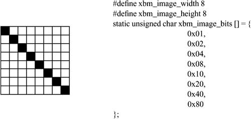
In the monochrome XBM format, the pixels of an image are encoded and written to a list of byte values (byte array) in the C programming language, grouping 8 pixels into a byte value. There are two additional definitions for the dimensions of an image (see Figure 4-3).
Figure 4-3 Example of an XBM image.
In XPM format, image data are encoded and written to a list of strings (string array), together with a header. The first line defines the image dimension and a hot spot, which is used as a cursor icon to identify the exact pixel that triggers a mouse selection. The next lines describe the colors used, replacing a text or an RGB color value by a character from the ASCII character set. The lines that follow these lines list the image lines, including their replaced color values (see Figure 4-4). Note that unused pixels are represented by blanks.
Figure 4-4 Example of an XPM image.

Neither XBM nor XPM images are compressed for storage. This means that their representation by 8-bit ASCII values generates always the same data volume. Both formats allow encoding of only 256 colors or gray levels.
4.2.2.7 Portable Bitmap plus (PBMplus)
PBMplus is a software package that allows conversion of images between various image formats and their script-based modification. PBMplus includes four different image formats, Portable Bitmap (PBM) for binary images, Portable Graymap (PGM) for gray-value images, Portable Pixmap (PPM) for true-color images, and Portable Anymap (PNM) for format-independent manipulation of images. These formats support both text and binary encoding. The software package contains conversion tools for internal graphic formats and other formats, so that it offers free and flexible conversion options.
The contents of PBMplus files are the following:
• A magic number identifying the file type (PBM, PGM, PPM, or PNM), that is, “P1” for PBM.
• Blanks, tabs, carriage returns, and line feeds.
• Decimal ASCII characters that define the image width.
• Decimal ASCII characters that define the image height.
• ASCII numbers plus blanks that specify the maximum value of color components and additional color information (for PPM, PNM, and PBM).
Filter tools are used to manipulate internal image formats. The functions offered by these tools include color reduction; quantization and analysis of color values; modification of contrast, brightness and chrominance; cutting, pasting and merging of several images; changing the size of images; or generating textures and fractal backgrounds.
4.2.2.8 Bitmap (BMP)
BMP files are device-independent bitmap files most frequently used in Windows systems. The BMP format is based on the RGB color model. BMP does not compress the original image. The BMP format defines a header and a data region. The header region (BITMAPINFO) contains information about size, color depth, color table, and compression method. The data region contains the value of each pixel in a line. Lines are flush-extended to a value divisible by 32 and padded with zero values.
Valid color depth values are 1, 4, 8, and 24. The BMP format uses the run-length encoding algorithm to compress images with a color depth of 4 or 8bits/pixel, where two bytes each are handled as an information unit. If the first byte value contains zero and the second value is greater than three, then the second value contains the number of bytes that follow and contains the color of the next pixel as a reference to the color table (no compression). Otherwise, the first byte value specifies the number of pixels that follow, which are to be replaced by the color of the second byte value to point to the color table. An image encoded with 4bits/pixel uses only four bits for this information. In the header region, BMP defines an additional option to specify a color table to be used to select colors when the image is displayed.
4.2.3 Creating Graphics
4.2.3.1 Input Devices
Modern graphical input devices include mice (with or without cables), tablets, and transparent, highly sensitive screens, or input devices that allow three-dimensional or higher-dimensional input values (degrees of freedom), in addition to the x and y positions on the screen, such as trackballs, spaceballs, or data gloves.
Some trackball models available today rotate around the vertical axis in addition to the two horizontal axes, but there is no direct relationship between hand movements on the device and the corresponding movement in three-dimensional space.
A spaceball is a solid ball positioned on an elastic base. Pressing or pulling the ball in any direction produces a 3D translation and a 3D orientation. The directions of movement correspond to the user’s attempts to move the solid ball although the hand does not actually move.
A data glove is a device that senses the hand position and its orientation [ZLB+87]. It allows pointing to objects, exploring and navigating within scenes, or acting at a distance on the real world. Virtual objects may be manipulated, for example rotated for further examination. With gloves, real objects may be moved at a distance, while the user only monitors their virtual representation. High-precision gloves are sophisticated and expensive instruments. Special gloves may feed back tactile sensations by means of “tactile corpuscles,” which exert pressure on the finger tips. Shapes of objects may thus be simulated. Research is also going on in the simulation of object textures.
4.2.3.2 Graphics Software
Graphics are generated by use of interactive graphic systems. The conceptual environment of almost all interactive graphic systems is an aggregated view consisting of three software components—application model, application program, and graphics system—and one hardware component.
The application model represents data or objects to be displayed on the screen. It is normally stored in an application database. The model acquires descriptions of primitives that describe the form of an object’s components, attributes, and relations that explain how the components relate to each other. The model is specific to an application and independent of a system used for display. This means that the application program has to convert a description of parts of the model into procedure calls or commands the graphic system can understand to create images. This conversion process is composed of two phases. First, the application program searches the application database for parts to be considered, applying certain selection or search criteria. Second, the extracted geometry is brought into a format that can be passed on to the graphics system.
The application program processes user input and produces views by sending a series of graphical output commands to the third component, the graphics system. These output commands include a detailed geometric description as to what is to be viewed and how the objects should appear.
The graphics system is responsible for image production involving detailed descriptions and for passing user input on to the application program (for processing purposes). Similar to an operating system, the graphics system represents an intermediate component between the application program and the display hardware. It influences the output transformation of objects of the application model into the model’s view. In a symmetric way, it also influences the input transformation of user actions for application program inputs leading to changes in the model and/or image. A graphics system normally consists of a set of output routines corresponding to various primitives, attributes, and other elements. The application program passes geometric primitives and attributes on to these routines. Subroutines control specific output devices and cause them to represent an image.
Interactive graphics systems are an integral part of distributed multimedia systems. The application model and the application program can represent applications as well as user interfaces. The graphics system uses (and defines) programming abstractions supported by the operating system to establish a connection to the graphics hardware.
4.2.4 Storing Graphics
Graphics primitives and their attributes are on a higher image representation level because they are generally not specified by a pixel matrix. This higher level has to be mapped to a lower level at one point during image processing, for example, when representing an image. Having the primitives on a higher level is an advantage, because it reduces the data volume that has to be stored for each image and allows simpler image manipulation. A drawback is that an additional step is required to convert graphics primitives and their attributes into a pixel representation. Some graphics packages, for example, the SRGP (Simple Raster Graphics Package), include this type of conversion. This means that such packages generate either a bitmap or a pixmap from graphics primitives and their attributes.
We have seen that a bitmap is a pixel list that can be mapped one-to-one to pixel screens. Pixel information is stored in 1 bit, resulting in a binary image that consists exclusively of black and white. The term pixmap is a more general description of an image that uses several bits for each pixel. Many color systems use 8 bits per pixel (e.g., GIF), so that 256 colors can be represented simultaneously. Other formats (including JPEG) allow 24 bits per pixel, representing approximately 16 million colors.
Other packages—for example, PHIGS (Programmer’s Hierarchical Interactive Graphics System) and GKS (Graphical Kernel System)—use graphics specified by primitives and attributes in pixmap form [FDFH92].
4.2.4.1 Graphics Storage Formats
File formats for vector graphics allow loading and storing of graphics in a vectored representation, such as files created in a vector graphics application. The most important file formats include:
• IGES: The Initial Graphics Exchange Standard was developed by an industry committee to formulate a standard for the transfer of 2D and 3D CAD data.
• DXF: AutoDesk’s 2D and 3D format was initially developed for AutoCAD, a computer-aided design application. It has become a de facto standard.
• HPGL: The Hewlett Packard Graphics Language has been designed to address plotters, which is the reason why it only supports 2D representation.
The combination of vector and raster graphics is generally possible in modern vector graphics systems. With regard to representing data in files, the two graphics types are often totally separated from one another. Only a few so-called meta file formats—for example, CGM (Computer Graphics Metafile), PICT (Apple Macintosh Picture Format), and WMF (Windows Metafile)—allow an arbitrary mixture of vector and raster graphics.
4.3 Computer-Assisted Graphics and Image Processing
Computer graphics deal with the graphical synthesis of real or imaginary images from computer-based models. In contrast to this technique, image processing involves the opposite process, that is, the analysis of scenes, or the reconstruction of models from images representing 2D or 3D objects. The following sections describe some image analysis (image recognition) and image synthesis (image generation) basics. For detailed information, see [FDFH92, KR82, Nev82, HS92, GW93].
4.3.1 Image Analysis
Image analysis involves techniques to extract descriptions from images, which are required by methods used to analyze scenes on a higher level. Knowing the position and the value of a particular pixel does not contribute enough information to recognize an object, to describe the object form and its position or orientation, to measure the distance to an object, or whether or not an object is defective. Techniques applied to analyzing images include the calculation of perceived colors and brightness, a partial or full reconstruction of three-dimensional data in a scene, and the characterization of the properties of uniform image regions.
Image analysis is important in many different fields, for example, to evaluate photos taken by an air contamination monitor, sampled TV pictures of the moon or other planets received from space probes, TV pictures generated by the visual sensor of an industrial robot, X-ray pictures, or CAT (Computerized Axial Tomography) pictures. Some image processing fields include image improvement, pattern discovery and recognition, scene analysis, and computer vision.
Image improvement is a technique to improve the image quality by eliminating noise (due to external effects or missing pixels), or by increasing the contrast.
Pattern discovery and pattern recognition involve the discovery and classification of standard patterns and the identification of deviations from these patterns. An important example is OCR (Optical Character Recognition) technology, which allows efficient reading of print media, typed pages, or handwritten pages into a computer. The degree of accuracy depends on the source material and the input device, particularly when reading handwritten pages. Some implementations allow users to enter characters by use of a steadily positioned device, normally a tablet pen, which are detected by the computer (online character recognition). This process is much easier compared to the recognition of scanned characters because the tablet acquires sequence, direction, and—in some cases—speed and pressure. Also, a pattern recognition algorithm can match these factors for each character against stored templates. The recognition process can evaluate patterns without knowing how the patterns have been created (static pattern recognition). Alternatively, it can respond to pressure, character edges, or the drawing speed (dynamic pattern recognition). For example, a recognition process can be trained to recognize various block capital styles. In such a process, the parameters of each character are calculated from patterns provided by the user. [KW93] describes an architecture of an object-oriented character recognition engine (AQUIRE), which supports online recognition with combined static and dynamic capabilities.
Scene analysis and computer vision concern the recognition and reconstruction of 3D models of a scene consisting of various 2D images. A practical example is an industrial robot that measures the relative sizes, shapes, positions, and colors of objects.
The following sections identify some properties that play an important role in recognizing images. Information yielded by these methods is subsequently aggregated to allow recognition of image contents.
4.3.1.1 Image Properties
Most image recognition methods use color, texture, and edges to classify images. Once we have described an image based on these three properties, we can, for example, query an image database by telling the system, “Find an image with a texture similar to that of the sample image.”
Color
One of the most intuitive and important characteristics to describe images is color. Assume that the image we want to analyze is available in the usual RGB format with three 8-bit color channels. The basic approach is to use a color histogram to acquire the image, that is, how many pixels of the image take a specific color. To avoid working with a indeterminable number of colors, we previously discretize the colors occurring in the image. We achieve this by using only the n leftmost bits of each channel. With n=2, our histogram will have entries for 64 colors. Figure 4-5 shows an example of a gray-value histogram (because this book is printed in black on white paper) for an image with a palette of 256 possible gray values.
Figure 4-5 The gray-value histogram of an image.

For humans to recognize the colorfulness of an image, it is relevant whether or not a color tends to occur on large surfaces (in a coherent environment) or in many small spots, in addition to the frequency in which a color occurs. This information will be lost if we were to count only the number of pixels in a specific color. For this reason, [PZM96] suggests a so-called color coherence vector (CCV). To calculate CCV, each pixel is checked as to whether it is within a sufficiently large one-color environment (i.e., in a region related by a path of pixels in the same color). If so, we call it coherent, otherwise it is incoherent. We prepare two separate histograms to count coherent and incoherent pixels for each color.
Assume we determined J colors after the discretization process, then αj or βj (j = 1, …, J) describe the number of coherent or incoherent pixels of the color j. The color coherence vector is then given by ((α1, β1), …, (αJ, βJ)), which we store to describe the colorfulness of the image. When comparing two images, B and B', against CCVs ((α1, β1), …, (αJ, βJ)) or ((α1', β1'), …, (αJ', βJ')), we use the expression

as a measure of distance.
An advantage of using color as our property to compare two images is that it is robust and can represent slight changes in scaling or perspective and it allows fast calculation. However, we cannot normally use the Euclidean distance of two color vectors to draw a direct conclusion on the difference in human color recognition. We can solve this problem by transforming the RGB image before we transform the histogram into a color space, which corresponds better to human recognition. One such color space is the so-called L*a*b* space (see [Sch97a]).
Texture
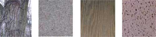
A texture is a small surface structure, either natural or artificial, regular or irregular. Examples of textures are wood barks or veining, knitting patterns, or the surface of a sponge, as shown in Figure 4-6. When studying textures, we distinguish between two basic approaches. First, the structural analysis searches for small basic components and an arrangement rule, by which to group these components to form a texture. Second, the statistical texture analysis describes the texture as a whole based on specific attributes, for example, local gray-level variance, regularity, coarseness, orientation, and contrast. These attributes are measured in the spatial domain or in the spatial frequency domain, without decoding the texture’s individual components. In practical applications, structural methods do not play an important role.
Figure 4-6 Some texture examples.
To analyze textures, color images are first converted into a gray-level representation. When studying natural images (e.g., landscape photographs), we have to deal with the issue of what structures we want to call a texture (which depends on the scaling and other factors) and where in the image there may be textured regions. To solve this issue, we can use a significant and regular variation of the gray values in a small environment [KJB96] as a criterion for the occurrence of a texture in an image region. Once we have opted for a texture measuring unit, we determine such homogeneous regions in the image segmentation process. Finally, we calculate the texture measuring unit for each texture region.
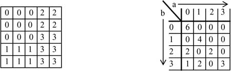
To illustrate this process, we use a simplified statistical method to analyze a texture in the local space. We calculate and interpret gray-level co-occurrence matrices [Zam89]. These matrices state how often two gray values, a and b, occur in an image in a specific arrangement. For an arrangement, [a][b] (i.e., gray-level b is immediately right of pixels with gray-level a), Figure 4-7 shows the gray-level co-occurrence matrix on the right for the sample represented on the left.
Figure 4-7 Example of a gray-level co-occurrence matrix.
We could form gray-level co-occurrence matrices for any other neighboring arrangement of two gray values. If we distinguish N gray values and call the entries in an N×N gray-level co-occurrence matrix g(a,b), then
![]()
can be used as a measurement unit for a texture’s contrast. Intuitively, we speak of high contrast when there are very different gray values in a dense neighborhood. If the gray levels are very different, (a-b)2, and if they border each other frequently, then g(a,b) takes a high value [Zam89]. It is meaningful not to limit to one single neighboring arrangement. The expression
![]()
measures a texture’s homogeneity, because in a homogeneous and perfectly regular texture, there are only very few different gray-level co-occurrence arrangements (i.e., essentially only those that occur in the small basic component), but they occur frequently.
Powerful texture analysis methods are based on multiscale simultaneous autoregression, Markov random fields, and tree-structured wavelet transforms. These methods go beyond the scope of this book; they are described in detail in [PM95, Pic96].
Edges
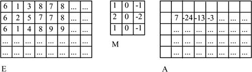
The use of edges to classify images provides a basic method for image analysis—the convolution of an image from a mask [Hab95]. This method uses a given input image, E, to gradually calculate a (zero-initialized) output image, A. A convolution mask (also called convolution kernel), M, runs across E pixel by pixel and links the entries in the mask at each position that M occupies in E with the gray value of the underlying image dots. The result of this linkage (and the subsequent sum across all products from the mask entry and the gray value of the underlying image pixel) is written to output image A. The terms
• e(x, y): gray value of the pixel at position (x, y) in input image E
• a(x, y): entry at position (x, y) in output image A
• m: size of mask M, that is, m×m, m uneven
• m(u, v): entry at position (u, v); u, v = 0, …, m-1 in mask M
are used to calculate k=(m-1)/2 from:
![]()
where marginal areas of width k remain initial in A. Figure 4-8 shows this method.
Figure 4-8 Using a filter.
This method is applied in the edge extraction process. A preliminary step smoothes the image available in gray-level representation, where the gray value of each pixel is replaced by a suitably weighed mean value of the gray values of its neighboring pixels, at the cost of losing some sharpness. However, this loss is tolerable because the method yields a less noisy image.
To locate pixels along the vertical edges (that is, pixels experiencing a strong horizontal gray-level transition), a mask, Mhoriz as shown in Figure 4-9, runs across the smoothed image. The Sobel operators used in this example are particularly suitable to locate gray-value transitions. In output image Ahoriz, a high-quantity entry means that there is a significant change in gray-levels in the “left-right direction” at the relevant position in E. The sign specifies the transition’s direction. The approach for the horizontal edges is similar; the convolution of E with Mvert results in Avert.
Figure 4-9 Using Sobel operators.

This concept provides partial derivations from E in the column and line directions. To determine the gradient amount that specifies the total strength of an “oblique” edge at position (x,y), we determine
![]()
and finally binarize the result by use of a threshold value, E. This means that only the pixels in which a sufficient gray-value gradient was determined will flow into the final output image. During binarization, 1s are entered for all pixels that exceed the threshold value and 0s are entered for all remaining pixels in the output image.
Subsequent steps involve calculation of the gradient orientation and determination of the quantities of pixels that are on the same edge.
4.3.1.2 Image Segmentation
Segmentation is an operation that assigns unique numbers (identifiers) to object pixels based on different intensities or colors in the foreground and background regions of an image. A zero is assigned to the background pixels. Segmentation is primarily used to identify related pixel areas, so-called objects, while the recognition of these objects is not part of the segmentation process.
The following example uses gray-level images, but the methods can be easily applied to color images by studying the R, G, and B components separately.
Segmentation methods are classified as follows [Bow92, Jäh97, Jai89, RB93, KR82]:
• Pixel-oriented methods
• Edge-oriented methods
• Region-oriented methods
In addition to these methods, many other methods are known [GW93, Fis97b], for example, methods working with neuronal networks.
Pixel-Oriented Segmentation Methods
The segmentation criterion in pixel-oriented segmentation is the gray value of a pixel studied in isolation. This method acquires the gray-level distribution of an image in a histogram and attempts to find one or several thresholds in this histogram [Jäh97, LCP90]. If the object we search has one color but a different background, then the result is a bimodal histogram with spatially separated maxima. Ideally, the histogram has a region without pixels. By setting a threshold at this position, we can divide the histogram into several regions.
Alternatively, we could segment on the basis of color values. In this case, we would have to modify the method to the three-dimensional space we study so that pixel clouds can be separated. Of course, locating a threshold value in a one-dimensional space of gray values is much easier. In practical applications, this method has several drawbacks:
• Bimodal distribution hardly occurs in nature, and digitization errors prevents bimodal distribution in almost all cases [Jäh97].
• If the object and background histograms overlap, then the pixels of overlapping regions cannot be properly allocated.
• To function properly, these methods normally require that the images be edited manually. This step involves marking the regions that can be segmented by use of local histograms.
Edge-Oriented Segmentation Methods
Edge-oriented segmentation methods work in two steps. First, the edges of an image are extracted, for example, by use of a Canny operator [Can86]. Second, the edges are connected so that they form closed contours around the objects to be extracted.
The literature describes several methods to connect edge segments into closed contours [GW93, KR82]. Many methods use the Hough transform to connect edges. This algorithm replaces a regression line by m predefined pixels, which means that the share of straight lines contained in an image can be determined in the image region.
The Hough transform is a technique that can be used to isolate features of a particular shape within an image. Because it requires that the desired features be specified in some parametric form, the classical Hough transform is most commonly used for the detection of regular curves such as lines, circles, ellipses, and so on. A generalized Hough transform can be employed in applications where a simple analytic description of features is not possible. Due to the computational complexity of the generalized Hough algorithm, we restrict the main focus of this discussion to the classical Hough transform. Despite its domain restrictions, the classical Hough transform retains many applications, as most manufactured parts (and many anatomical parts investigated in medical imagery) contain feature boundaries that can be described by regular curves. The main advantage of the Hough transform technique is that it is tolerant of gaps in feature boundary descriptions and is relatively unaffected by image noise.
The Hough technique is particularly useful for computing a global description of a feature (where the number of solution classes need not be known a priori), given (possibly noisy) local measurements.
As a simple example, Figure 4-10 shows a straight line and the pertaining Hough transform. We use the Hough transform to locate straight lines contained in the image. These lines provide hints as to how the edges we want to extract can be connected. To achieve this goal, we take the straight lines starting at one edge end in the Hough transform to the next edge segment into the resulting image to obtain the contours we are looking for.
Figure 4-10 Using the Hough transform to segment an image.

Once we have found the contours, we can use a simple region-growing method to number the objects. The region-growing method is described in the following section.
Region-Oriented Segmentation Methods
Geometric proximity plays an important role in object segmentation [CLP94]. Neighboring pixels normally have similar properties. This aspect is not taken into account in the pixel- and edge-oriented methods. In contrast, region-growing methods consider this aspect by starting with a “seed” pixel. Successively, the pixel’s neighbors are included if they have some similarity to the seed pixel. The algorithm checks on each k level and for each region ![]() of the image’s N regions whether or not there are unqualified pixels in the neighborhood of the marginal pixels. If an unqualified marginal pixel, x, is found, then the algorithm checks whether or not it is homogeneous to the region to be formed.
of the image’s N regions whether or not there are unqualified pixels in the neighborhood of the marginal pixels. If an unqualified marginal pixel, x, is found, then the algorithm checks whether or not it is homogeneous to the region to be formed.
For this purpose, we use homogeneity condition ![]() = TRUE. For example, to check homogeneity P, we can use the standard deviation of the gray levels of one region.
= TRUE. For example, to check homogeneity P, we can use the standard deviation of the gray levels of one region.
Ideally, one seed pixel should be defined for each region. To automate the seed pixel setting process, we could use the pixels that represent the maxima from the histograms of the gray-level distribution of the images [KR82].
An efficient implementation of the required algorithm works recursively. Assume that a function, ELEMENT, is defined. The function specifies whether or not the homogeneity condition is met and one pixel has been marked. The steps involved in this algorithm are the following:
FUNCTION regionGrowing(x,y)
if (ELEMENT(x,y))
mark pixel as pertaining to object
else
if (ELEMENT(x-1,y-1)) regionGrowing(x-1,y-1)
if (ELEMENT(x-1,y)) regionGrowing(x-1,y)
if (ELEMENT(x-1,y+1)) regionGrowing(x-1,y+1)
if (ELEMENT(x,y-1)) regionGrowing(x,y-1)
if (ELEMENT(x,y+1)) regionGrowing(x,y+1)
if (ELEMENT(x+1,y-1)) regionGrowing(x+1,y-1)
if (ELEMENT(x+1,y)) regionGrowing(x+1,y)
if (ELEMENT(x+1,y+1)) regionGrowing(x+1,y+1)
A drawback of this algorithm is that it requires a large stack region. If the image consists of one single object, we need a stack size corresponding to the image size. With a 100×100-pixel image, we would need a stack with a minimum depth of 10,000 pixels. Note that the stack depth of modern workstations is much smaller. For this reason, a less elegant iterative variant [FDFH92] is often used.
Region growing is based on a bottom-up approach, because smallest image regions grow gradually into larger objects. A drawback of this method is its high computing requirement. This problem can be solved by the split-and-merge algorithm—an efficient top-down algorithm [BD97, CMVM86, CP79], however at the cost of losing contour sharpness. The split step studies a square region as to homogeneity.
The gray-level mean value of a region is often used as a homogeneity criterion:

with standard deviation
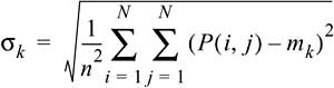
where a region, k, is homogeneous with regard to a threshold, T, if σk < T.
Selecting threshold value T enables us to determine the granularity of the segmentation result. An inhomogeneous region is divided into four equally sized subregions and the process is repeated. However, this process may produce neighboring and homogeneous regions, which have to be merged in the subsequent merge step.
If (|m1 - m2| < k × σi, i = 1, 2), we can merge two regions, where k serves as a factor specifying the granularity of the segmented image. Figure 4-11 shows this algorithm.
Figure 4-11 Using the split-and-merge algorithm.

Edge-oriented segmentation does not take interrelationships between regions into account during segmentation, that is, it utilizes only local information. The region-growing algorithm makes efficient use of pixel relationships, which means that it utilizes global information. On the other hand, it does not make efficient use of local edge information.
Ongoing work attempts to solve the discrepancy problem between the two approaches [Fis97a, Hen95]. The following section describes an algorithm that combines both approaches.
Water-Inflow Segmentation
The previous sections described local and global segmentation strategies. A more efficient segmentation can be achieved by combining the local and global approaches [HB90, Hen95, PL90, Fis97a]. The example given in this section uses the so-called water-inflow algorithm [Fis97a].
The basic idea behind the water-inflow method is to fill a gray-level image gradually with water. During this process, the gray levels of the pixels are taken as height. The higher the water rises as the algorithm iterates, the more pixels are flooded. This means that land and water regions exist in each of the steps involved. The land regions correspond to objects. The second steps unifies the resulting segmented image parts into a single image. This method is an expansion of the watershed method introduced by Vincent and Soille [VS91]. Figure 4-12 shows the segmentation result at water level 30.
Figure 4-12 Segmentation result at a specific water level.

One advantage of this approach is that depth information lost when matching three-dimensional real-world images with two-dimensional images can be recovered, at least in part. Assume we look at a bent arm. Most segmentation strategies would find three objects: the upper part of the body, the arm, and the lower part of the body (which implies that the arm has a different gray level than the rest of the body). The water-inflow algorithm can recognize that the arm is in front of the body, from a spatial view. For this view, we need to create a hierarchy graph.
Now let’s see how this algorithm works. First, it finds large objects, which are gradually split into smaller objects as the algorithm progresses. (The first object studied is the complete image.) This progress can be represented in a hierarchical graph. The root of the graph is the entire image. During each step, while objects are cloned, more new nodes are added to the graph. As new nodes are added, they become the sons of the respective object nodes. These nodes store the water level found for an object and a seed pixel for use in the region-growing process. This arrangement allows relocation of an arbitrary subobject when needed. The different gray levels of the subobjects ensure that the subobjects can be recognized as the water level rises and the algorithm progresses.
This means that, by splitting objects into smaller objects, we obtain an important tool to develop an efficient segmentation method. This aspect is also the main characteristic of this approach versus the methods described earlier.
4.3.1.3 Image Recognition
Previous sections described properties that can be used to classify the content of an image. So far, we have left out how image contents can be recognized. This section describes the entire process required for object recognition.
The complete process of recognizing objects in an image implies that we recognize a match between the sensorial projection (e.g., by a camera) and the observed image. How an object appears in an image depends on the spatial configuration of the pixel values. The following conditions have to be met for the observed spatial configuration and the expected projection to match:
• The position and the orientation of an object can be explicitly or implicitly derived from the spatial configuration.
• There is a way to verify that the derivation is correct.
To derive the position, orientation, and category or class of an object (e.g., a cup) from the spatial configuration of gray levels, we need a way to determine the pixels that are part of an object (as described in the segmentation section). Next, we need a way to distinguish various observed object characteristics from the pixels that are part of an object, for example, special markings, lines, curves, surfaces, or object boundaries (e.g., the rim of a cup). These characteristics are, in turn, organized in a spatial image-object relationship.
The analytical derivation of form, position, and orientation of an object depends on whether various object characteristics (a dot, line segment, or region in the two-dimensional space) match with corresponding object properties (a dot, line segment, circle segment, or a curved or plane surface).
The types of object, background, or sensor used to acquire the image, and the sensor’s location determine whether a recognition problem is difficult or easy. Take, for example, a digital image with an object in the form of a white plane square on an evenly black background (see Table 4-1).
Table 4-1 Numeric digital intensity image with a white square (gray level FF) on black background (gray level 0) of a symbolic image.
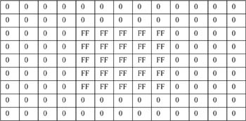
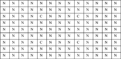
A simple edge extraction method or a segmentation method could find the corner points (see Table 4-2). In this case, there is a direct match between the characteristics of the corners in the image and those of the object corners.
Table 4-2 Numeric digital intensity image of the corners of the image from Table 4-1 (C = corner; N = no corner).
However, a transformation process may be difficult. It may involve the recognition of a series of complex objects. Also, some objects could contain parts of other objects, there could be shadows, the light reflected by the object could vary, or the background could be restless.
The decision as to what type of transformation is suitable depends on the specific nature of the observation task, the image complexity, and the type of information available at the beginning.
In general, computer-supported object recognition and inspection is a complex task. It involves a number of different steps to successively transform object data into recognition information. To be suitable, a recognition method should include the following six steps: image formatting, conditioning, marking, grouping, extraction, and matching. These steps are shown schematically in Figure 4-13 and described briefly in the following section.
Figure 4-13 Steps involved in image recognition.

The Image-Recognition Procedure
This section provides a brief introduction to the image recognition steps. A detailed analysis is given in [Nev82, HS92] and [GW93].
The formatting step shoots an image by use of a camera and transforms the image into digital form (i.e., pixels as described above). The conditioning, marking, grouping, extraction, and matching steps form a canonic division of the image recognition problem, where each step prepares and transforms the data required for the next step. Depending on the application, it may be necessary to apply this sequence to more than one level of recognition and description. These five steps are:
1. Conditioning: Conditioning is based on a model that assumes an image that can be observed is composed of information patterns, which are disturbed by irrelevant variations. Such variations are typically additive or multiplicative parts of such a pattern. Conditioning estimates the information pattern based on the observed image, so that noise (an unwanted disturbance that can be seen as a random change without recognizable pattern and that falsifies each measurement) can be suppressed. Also, conditioning can normalize the background by ignoring irrelevant systematic or patterned variations. The typical conditioning process is independent from the context.
2. Marking: Marking is based on a model that assumes that information patterns have a structure in the form of spatial object arrangements, where each object is a set of interconnected pixels. Marking determines to which spatial objects each pixel belongs.
An example of a marking operation is the edge recognition method described above. Edge recognition techniques find local discontinuities of some image attributes, such as intensity or color (e.g., the rim of a cup). These discontinuities are particularly interesting because there is a high probability that they occur along the boundaries of an object. Edge recognition finds a large quantity of edges, but not all of them are significant. For this reason, an additional marking operation has to be used after the edge recognition. This operation is called thresholding; it specifies the edges that should be accepted and those that can be discarded. This means that the operation filters and marks the significant edges of an image, while the remaining edges are removed. Additional marking operations can find corner dots.
3. Grouping: The grouping operation identifies objects marked in the previous step by grouping pixels that are part of the same object, or by identifying maximum quantities of interconnected pixels. Considering that intensity-based edge recognition is actually a gradual modification, the grouping step includes the edge connection step. A grouping operation that groups edges into lines is also called line fitting, for which the above described Hough transform and other transform methods can be used.
The grouping operation changes the logical data structure. The original images, the conditioned, and marked images are all available as digital image data structures. Depending on the implementation, the grouping operation can produce either an image data structure in which an index is assigned to each pixel and the index is associated with this spatial occurrence, or a data structure that represents a quantity collection. Each quantity corresponds to a spatial occurrence and contains line/column pairs specifying the position, which are part of the occurrence. Both cases change the data structure. The relevant units are pixels before and pixel quantities after the grouping operation.
4. Extraction: The grouping operation defines a new set of units, but they are incomplete because they have an identity but no semantic meaning. The extraction operation calculates a list of properties for each pixel group. Such properties can include center (gravity), surface, orientation, spatial moments, spatial grayscale moments, and circles. Other properties depend on whether the group is seen as a region or as a circle sector. For a group in the form of a region, the number of holes in the interconnected pixel group could be a meaningful property. On the other hand, the mean curvature could be a meaningful indicator for a circle section.
In addition, the extraction operation can measure topological or spatial relationships between two or more groups. For example, it could reveal that two groups touch each other, or that they are close spatial neighbors, or that one group has overlaid another one.
5. Matching: When the extraction operation is finished, the objects occurring in an image are identified and measured, but they have no content meaning. We obtain a content meaning by attempting an observation-specific organization in such a way that a unique set of spatial objects in the segmented image results in a unique image instance of a known object, for example, a chair or the letter “A”. Once an object or a set of object parts has been recognized, we can measure things like the surface or distance between two object parts or the angles between two lines. These measurements can be adapted to a given tolerance, which may be the case in an inspection scenario. The matching operation determines how to interpret a set of related image objects, to which a given object of the three-dimensional world or a two-dimensional form is assigned.
While various matching operations are known, the classical method is template matching, which compares a pattern against stored models (templates) with known patterns and selects the best match.
4.3.2 Image Synthesis
Image synthesis is an integral part of all computer-supported user interfaces and a necessary process to visualize 2D, 3D, or higher-dimensional objects. A large number of disciplines, including education, science, medicine, construction, advertising, and the entertainment industry, rely heavily on graphical applications, for example:
• User interfaces: Applications based on the Microsoft Windows operating system have user interfaces to run several activities simultaneously and offer point-and-click options to select menu items, icons, and objects on the screen.
• Office automation and electronic publishing: The use of graphics in the production and distribution of information has increased dramatically since desktop publishing was introduced on personal computers. Both office automation and electronic publishing applications can produce printed and electronic documents containing text, tables, graphs, and other types of drawn or scanned graphic elements. Hypermedia systems allow viewing of networked multimedia documents and have experienced a particularly strong proliferation.
• Simulation and animation for scientific visualization and entertainment: Animated movies and presentations of temporally varying behavior of real and simulated objects on computers have been used increasingly for scientific visualization. For example, they can be used to study mathematical models of phenomena, such as flow behavior of liquids, relativity theory, or nuclear and chemical reactions. Cartoon actors are increasingly modeled as three-dimensional computer-assisted descriptions. Computers can control their movements more easily compared to drawing the figures manually. The trend is towards flying logos or other visual tricks in TV commercials or special effects in movies.
Interactive computer graphics are the most important tool in the image production process since the invention of photography and television. With these tools, we cannot only create images of real-world objects, but also abstract, synthetic objects, such as images of mathematical four-dimensional surfaces.
4.3.2.1 Dynamic Versus Static Graphics
The use of graphics is not limited to static images. Images can also vary dynamically. For example, a user can control an animation by adjusting the speed or changing the visible part of a scene or a detail. This means that dynamics are an integral part of (dynamic) graphics. Most modern interactive graphics technologies include hardware and software allowing users to control and adapt the dynamics of a presentation:
• Movement dynamics: Movement dynamics means that objects can be moved or activated relative to a static observer’s viewpoint. Objects may also be static while their environment moves. A typical example is a flight simulator containing components that support a cockpit and an indicator panel. The computer controls the movement of the platform, the orientation of the aircraft, and the simulated environment of both stationary and moving objects through which the pilot navigates.
• Adaptation dynamics: Adaptation dynamics means the current change of form, color, or other properties of observed objects. For example, a system could represent the structural deformation of an aircraft in the air as a response to many different control mechanisms manipulated by the user. The more subtle and uniform the change, the more realistic and meaningful is the result. Dynamic interactive graphics offer a wide range of user-controllable modes. At the same time, these modes encode and convey information, for example, 2D or 3D forms of objects in an image, their gray levels or colors, and the temporal changes of their properties.
4.4 Reconstructing Images
We said at the beginning of this chapter that a two-dimensional image signal taken by a camera is built by projecting the spatial (three-dimensional) real world onto the two-dimensional plane. This section introduces methods used to reconstruct the original three-dimensional world based on projection data. To reconstruct an image, we normally need a continuous series of projection images. The methods used to reconstruct images include the Radon transform and stereoscopy, which will be described briefly below.
4.4.1 The Radon Transform
Computer tomography uses pervious projections, regardless of whether or not an image is obtained from X-rays, ultrasound, magnetic resonance, or nuclear spin effects. The intensity of the captured image depends mainly on the “perviousness” of the volume exposed to radiation. A popular method used in this field is the Radon transform [Jäh97].
To understand how this method works, assume that the equation of a straight line across A and B runs at a distance d1 and at an angle θ to the origin of d1 = r cosθ + s sinθ.
We can form the integral of “brightness” along this beam by utilizing the fade-out property of the delta function, which is all zeros, except in the respective position, (r, s):

Figure 4-14 Using the Radon transform.

If we operate this transform on a variable instead of a fixed distance, d1, we obtain the continuous two-dimensional Radon transform x(θ, d) from x(r,s). Two variants of the Radon transform are in use: parallel-beam projection and fan-beam projection x(θ, t), which is based on a punctual radiation source, where angle β has to be defined for each single beam.
In addition, the method shows that the 1D Fourier transform of a Radon transform is directly related to the 2D Fourier transform of the original image in all possible angles θ (this is the projection disk theorem):
F(u,v) = F{x(r,s)}; F(θ,w) = F{Rx(θ,t)}
F(u,v) = F(θ,w) for u = w cosθ, v = w sinθ
We can now clearly reconstruct the image signal from the projection:

However, reconstruction will be perfect only for the continuous case. In the discrete case, the integrals flow into sums. Also, only a limited number of projection angles is normally available, and inter-pixel interpolations are necessary. As a general rule, reconstruction improves (but gets more complex) as more information becomes available and the finer the sampling in d and θ (and the more beams available from different directions).
4.4.2 Stereoscopy
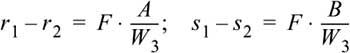
Objects in natural scenes observed by humans are normally not transparent; instead, we see only their surfaces. The Radon transform does not make sense in this case, because only the brightness of a single point will flow into the projection. The principle of stereoscopy, which is necessary in order to be able to determine the spatial distance, is based on the capture of two “retinal beams.” This process typically involves a central projection equation and two cameras. Assume that one camera is positioned at W1=0, W2=0, W3=0 and the second at W1=A, W2=B, W3=0. Further assume that a point, P, of the world coordinate [W1, W2, W3] is in the image level of the first camera at position [r1, s1] and for the second camera at position [r2, s2]. Using the central projection equation, we obtain
![]()
Assuming that both cameras have the same focal length, F, we obtain the distance of point P in W3:
![]()
The relative shift between the observation points on the image levels of a camera is called stereoscopic parallax:
The stereoscopic parallax is proportionally inverse to the distance of the point observed by the cameras. We now obtain
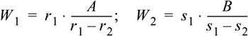
This example shows that it is not difficult to produce an exact image of the three-dimensional space. However, the process is limited, for example with regard to the estimated height (W2), when B is very small (both eyes or cameras are at same height). Another problem is that we always have to produce an exact point-by-point correspondence between the image dots captured by the cameras, which is not possible along the object boundaries, where the background may be obstructed for one camera but not for the other one (see Figure 4-15). Yet another problem is that camera and reflection noise may cause differences in the local brightness.
Figure 4-15 Stereovision.
4.5 Graphics and Image Output Options
Modern visual output technologies use raster display devices that display primitives in special buffers called refresh buffers in the form of pixel components. Figure 4-16 shows the architecture of a raster display device.
Some raster display devices have a display controller in hardware that receives and interprets output command sequences. In low-end systems, for example, personal computers (as in Figure 4-16), the display controller is implemented in software and exists as a component of a graphics library. In this case, the refresh buffer is part of the CPU memory. The video controller can read this memory to output images.
The complete display of a raster display device is formed by the raster, consisting of horizontal raster lines that are each composed of pixels. The raster is stored in the form of a pixel matrix that represents the entire screen area. The video controller samples the entire screen line by line.
Figure 4-16 Architecture of a raster display device.

Raster graphics can represent areas filled with colors or patterns, for example, realistic images of three-dimensional objects. The screen refresh process is totally independent of the image complexity (e.g., number of polygons), because modern hardware works fast enough to read each pixel from the buffer in every refresh cycle.
4.5.1 Dithering
Raster graphics technology has been developed at a fast pace, so that all modern computer graphics can represent color and gray-level images. The color depends primarily on the object, but also on light sources, environment colors, and human perception. On a black-and-white TV set or computer monitor, we perceive achromatic light, which is determined by the light quality. Light quality is an attribute determined by brightness and luminance parameters.
State-of-the-art technology uses the capabilities of the human eye to provide spatial integration. For example, if we perceive a very small area at a sufficiently long distance, our eyes form a mean value of fine-granular details of that small area and acquire only its overall intensity. This phenomenon is called continuous-tone approximation (dithering by means of grouped dots). This technique draws a black circle around each smallest resolution unit, where the circle’s surface is proportional to the blackness, 1-I (I stands for intensity), of the original picture surface. Image and graphics output devices can approximate variable surface circles for continuous-tone reproduction. To understand how this works, imagine a 2×2-pixel surface displayed on a monitor that supports only two colors to create five different gray levels at the cost of splitting the spatial resolution along the axes into two halves. The patterns shown in Figure 4-17 can be filled with 2×2 surfaces, where the number of enabled pixels is proportional to the desired intensity. The patterns can be represented by a dithering matrix.
Figure 4-17 Using 2×2 dithering patterns to approximate five intensity levels.

This technique is used by devices that cannot represent individual dots (e.g., laser printers). Such devices produce poor quality if they need to reproduce enabled isolated pixels (the black dots in Figure 4-17). All pixels enabled for a specific intensity must be neighbors of other enabled pixels.
In contrast, a CRT display unit is capable of representing individual dots. To represent images on a CRT display unit, the grouping requirement is less strict, which means that any dithering method based on a finely distributed dot order can be used. Alternatively, monochrome dithering techniques can be used to increase the number of available colors at the cost of resolution. For example, we could use 2×2 pattern surfaces to represent 125 colors on a conventional color screen that uses three bits per pixel—one each for red, green, and blue. Each pattern can represent five intensities for each color by using the continuous-tone pattern shown in Figure 4-17, so that we obtain 5×5×5 = 125 color combinations.
4.6 Summary and Outlook
This chapter described a few characteristics of images and graphics. The quality of these media depends on the quality of the underlying hardware, such as digitization equipment, monitor, and other input and output devices. The development of input and output devices progresses quickly. Most recent innovations include new multimedia devices and improved versions of existing multimedia equipment. For example, the most recent generation of scanners for photographs supports high-quality digital images. Of course, such devices are quickly embraced by multimedia applications. On the other hand, the introduction of new multimedia devices (e.g., scanners) implies new multimedia formats to ensure that a new medium (e.g., photographs) can be combined with other media. One example is Kodak’s introduction of their Photo Image Pac file format. This disk format combines high-resolution images with text, graphics, and sound. It allows the development of interactive photo-CD-based presentations [Ann94b]. (Optical storage media are covered in Chapter 8.)
Most existing multimedia devices are continually improved and new versions are introduced to the market in regular intervals. For example, new 3D digitization cards allow users to scan 3D objects in any form and size into the computer [Ann94a].