
The concept of competitive learning combined with neighborhood neurons gives us Kohonen SOMs. Every neuron in the output layer has two neighbors. The neuron that fires the greatest value updates its weights in competitive learning, but in SOM, the neighboring neurons also update their weights at a relatively slow rate. The number of neighborhood neurons that the network updates the weights is based on the dimension of the problem.
For a 2D problem, the SOM is represented as follows:
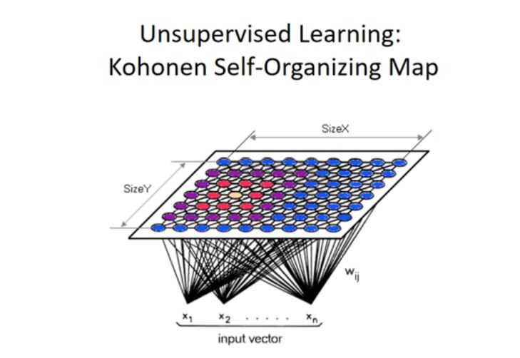
Diagrammatically, this is how the SOM maps different colors into different clusters:

Let us understand the working of Kohonen SOM step-by-step:
- The number of inputs and the clusters that define the SOM structure and each node's weights are initialized.
- A vector is chosen at random from the set of training data and is presented to the network.
- Every node in the network is examined to calculate which one's weights are most similar to the input vector. The winning node is commonly known as the Best Matching Unit (BMU).
- The radius of the neighborhood of the BMU is calculated. This value starts large and is typically set to be the radius of the network, diminishing each time-step.
- Any neurons found within the radius of the BMU, calculated in step 4, are adjusted to make them more like the input vector. The closer a neuron is to the BMU, the more its weights are altered.
- Repeat from step 2 for N iterations.
The steps are repeated for a set of N epochs or until a minimum weight update is obtained.
SOMs are used in the fields of clustering (grouping of data into different buckets), data abstraction (deriving output data from inputs), and dimensionality reduction (reducing the number of input features). SOMs handle the problem in a way similar to Multi Dimensional Scaling (MDS), but instead of minimizing the distances, they try regroup topology, or in other words, they try to keep the same neighbors.
Let us see an example of SOM implementation in R. The kohonen package is a package to be installed to use the functions offered in R for SOM.
The following R program explains some functions from the kohonen package :
######################################################################
###Chapter 2 - Introduction to Neural Networks - using R    ##########
###Usuervised ML technique using Kohonen package  ####################
######################filename: kohonen.r#############################
######################################################################
library("kohonen")

data("wines")
str(wines)
head(wines)
View (wines)

set.seed(1)
som.wines = som(scale(wines), grid = somgrid(5, 5, "hexagonal"))
som.wines
dim(getCodes(som.wines))

plot(som.wines, main = "Wine data Kohonen SOM")
par(mfrow = c(1, 1))
plot(som.wines, type = "changes", main = "Wine data: SOM")

training = sample(nrow(wines), 150)
Xtraining = scale(wines[training, ])
Xtest = scale(wines[-training, ],
              center = attr(Xtraining, "scaled:center"),
              scale = attr(Xtraining, "scaled:scale"))
trainingdata = list(measurements = Xtraining,
              vintages = vintages[training])
testdata = list(measurements = Xtest, vintages = vintages[-training])
mygrid = somgrid(5, 5, "hexagonal")
som.wines = supersom(trainingdata, grid = mygrid)

som.prediction = predict(som.wines, newdata = testdata)
table(vintages[-training], som.prediction$predictions[["vintages"]])
######################################################################
The code uses a wine dataset, which contains a data frame with 177 rows and 13 columns; the object vintages contains the class labels. This data is obtained from the chemical analyses of wines grown in the same region in Italy (Piemonte) but derived from three different cultivars, namely, the Nebbiolo, Barberas, and Grignolino grapes. The wine from the Nebbiolo grape is called Barolo. The data consists of the amounts of several constituents found in each of the three types of wines, as well as some spectroscopic variables.
Now, let's see the outputs at each section of the code.
library("kohonen")
The first line of the code is simple, as it loads the library we will use for later calculations. Specifically, the kohonen library will help us to train SOMs. Also, interrogation of the maps and prediction using trained maps are supported.
data("wines")
str(wines)
head(wines)
view (wines)
These lines load the wines dataset, which, as we anticipated, is contained in the R distribution, and saves it in a dataframe named data. Then, we use the str function to view a compactly display the structure of the dataset. The function head is used to return the first or last parts of the dataframe. Finally, the view function is used to invoke a spreadsheet-style data viewer on the dataframe object, as shown in the following figure:

We will continue to analyze the code:
set.seed(1)
som.wines = som(scale(wines), grid = somgrid(5, 5, "hexagonal"))
dim(getCodes(som.wines))
plot(som.wines, main = "Wine data Kohonen SOM")
After loading the wine data and setting seed for reproducibility, we call som to create a 5x5 matrix, in which the features have to be clustered. The function internally does the kohonen processing and the result can be seen by the clusters formed with the features. There are 25 clusters created, each of which has a combined set of features having common pattern, as shown in the following image:

The next part of the code plots the mean distance to the closest unit versus the number of iterations done by som:
graphics.off()
par(mfrow = c(1, 1))
plot(som.wines, type = "changes", main = "Wine data: SOM")
In the following figure is shown mean distance to closest unit versus the number of iterations:

Next, we create a training dataset with 150 rows and test dataset with 27 rows. We run the SOM and predict with the test data. The supersom function is used here. Here, the model is supervised SOM:
training = sample(nrow(wines), 150)
Xtraining = scale(wines[training, ])
Xtest = scale(wines[-training, ],
              center = attr(Xtraining, "scaled:center"),
              scale = attr(Xtraining, "scaled:scale"))
trainingdata = list(measurements = Xtraining,
                    vintages = vintages[training])
testdata = list(measurements = Xtest, vintages = vintages[-training])
mygrid = somgrid(5, 5, "hexagonal")
som.wines = supersom(trainingdata, grid = mygrid)

som.prediction = predict(som.wines, newdata = testdata)
table(vintages[-training], som.prediction$predictions[["vintages"]])
Finally, we invoke the table function that uses the cross-classifying factors to build a contingency table of the counts at each combination of factor levels, as shown next:
> table(vintages[-training], som.prediction$predictions[["vintages"]])

              Barbera Barolo Grignolino
 Barbera            5      0          0
 Barolo             0     11          0
 Grignolino         0      0         11
The kohonen package features standard SOMs and two extensions: for classification and regression purposes, and for data mining. Also, it has extensive graphics capability for visualization.
The following table lists the functions available in the kohonen package:
| Function name | Description |
| som | Standard SOM |
| xyf, bdk | Supervised SOM; two parallel maps |
| supersom | SOM with multiple parallel maps |
| plot.kohonen | Generic plotting function |
| summary.kohonen | Generic summary function |
| map.kohonen | Map data to the most similar neuron |
| predict.kohonen | Generic function to predict properties |