
4
Polynomial Interpolation
4.0 INTRODUCTION
Let ![]() be a function of x. Suppose we are given a set of value of y, say
be a function of x. Suppose we are given a set of value of y, say ![]() corresponding to given values of x, say x0, x1, x2, …, xi, …, xn. The values of x are called arguments and values of y are called entries.
corresponding to given values of x, say x0, x1, x2, …, xi, …, xn. The values of x are called arguments and values of y are called entries.
Interpolation may be defined as the process of finding the values of a function f(x) for any intermediate value of the argument x between x0 and xn. This process has been described by Thiele as “the art of reading between the lines of a table”.
In the broader sense interpolation is the process of replacing the unknown function or complicated function f(x) by a simpler function ϕ(x) which assumes the same values of y for the given values of x. The function ϕ(x) is called the interpolating function or interpolating formula. In many engineering applications this function is called a smoothing function.
A desirable characteristic of interpolating function is that it must be simple. Since polynomials are the simplest of the functions, we usually choose ϕ(x) to be a polynomial and so it is called interpolating polynomial. Nearly all the standard formulae of interpolation are polynomials. In case the given values indicate that the function is periodic, we represent it by a finite trigonometric series. But we consider here only polynomial interpolation.
The process of representing by a polynomial is justified by the Weierstrass theorem: “Every function f(x), which is continuous in an interval (a,b) can be represented in that interval, to any desired degree of accuracy by a polynomial ϕ(x)”.
Some of the important interpolating polynomial formulae are
- Newton’s forward and backward formulae
- Newton’s divided difference formula
- Lagrange’s formula
- The central difference formulae
- Gauss forward and backward formulae
- Stirling’s formula
- Everrett’s formula
- Bessel’s formula etc
All these formulae are expressed interms of difference operators of various types. So we shall first introduce the different difference operators.
Extrapolation: The process of obtaining the value of a tabulated function outside the interval of the given values of the arguments is called extrapolation or prediction.
4.1 FINITE DIFFERENCE OPERATORS
When the changes in the independent variable or argument of a function is discrete, the infinitesimal calculus cannot be applied to study such functions. But the calculus of finite differences enable us to study such functions. The calculus of finite differences form the basis of many processes and is used in the derivation of many formulae in numerical analysis.
4.1.1 Forward Difference Operator Δ
Let y0, y1, y2,…, yn be the values of the function ![]() at equally spaced arguments x0, x1, x2,…, xn respectively.
at equally spaced arguments x0, x1, x2,…, xn respectively.
Let the equal space or interval be h.
Then ![]()
![]()
Consider the differences ![]()
We denote these as
![]()
and are called first order forward differences or first differences and Δ is called the forward difference operator.
The difference of first order differences are called second order differences.
They are
![]()
Similarly we can find 3rd, 4th, …, nth order differences.
Thus
![]()
If ![]() , then
, then ![]()
![]()
Forward difference table

The first entry y0 is called the leading term and the differences ![]() in the diagonal through y0 are called the leading differences.
in the diagonal through y0 are called the leading differences.
4.1.2 Backward Difference Operator ∇ (Read as Del or Nebla)
The differences ![]() are denoted by
are denoted by ![]() and are called first order backward differences. The operator ∇ is called backward difference operator.
and are called first order backward differences. The operator ∇ is called backward difference operator.
∴ ![]()
The differences
![]()
are called second order backward differences and so on.
![]()
The backward difference table is

Prove that ![]()
Prove:
We have
![]()


Similarly
![]()
4.1.3 Shift Operator or Displacement Operator E
The operator E is defined by ![]() where h is the interval of differencing. That is E shifts
where h is the interval of differencing. That is E shifts ![]() to next higher value
to next higher value ![]()
In other words ![]() , where
, where ![]() and
and ![]()

The operator ![]() is defined as
is defined as ![]() , where h is the interval of differencing.
, where h is the interval of differencing.
That is ![]() shifts
shifts ![]() to preceeding lower value
to preceeding lower value ![]() .
.
In other words, ![]() where
where ![]() and
and ![]()

Note: ![]() and
and ![]() where 1 is the identity operator
where 1 is the identity operator
4.1.4 Relation Between the Operators E, Δ, ∇
- Prove that
 where 1 is the identity operator.
Proof:
We have

and


∴
 for any
∴

Similarly
 ,
,
Note: The method of writing the operator equality is known as the method of separation of symbols. However it should be remembered that operators cannot really stand alone and the operand
 is always understood.
 - Prove that

Proof:
We have

and


∴
 for any
∴

4.1.5 Properties of Δ and E
- Δ is linear operator
ie.

and
 , where C is a constant.
 - E is a linear operator
ie.

and

- Index laws
If m and n are positive integers, then

Similarly

 is the inverse operator of
 is the inverse operator of
- Prove that Δ∇ = ∇Δ
Proof:
We have


⇒


- Prove that

Proof:
We have

and


∴
 for any
∴

- Prove that

Proof:
We have


∴
 for any
⇒

Because of this property, we shall write each side

Theorem 4.1
The nth differences of a polynomial of nth degree are constant.
ie. If
 is an nth degree polynomial, then
  constant, where h is the interval of differencing.
Note:
 More generally,
- The converse of this theorem is also true.
That is, if the nth differences of a function tabulated at equally spaced arguments are constants, then the function is a polynomial of nth degree.
The Converse is of great use in practical situations. If in a difference table the nth differences are constant or nearly so (since rounding off errors may prevent them being exactly equal), then the function may be represented by a polynomial of nth degree by a suitable interpolation formula.
- The Central difference operator
The Central difference operator δ is defined by
 .
.
- The averaging operator or the mean value operator μ is defined by


- Prove that

Proof:


- Prove that

Proof:
We have
 (1)
(1)and


- Relation between differentical operator and difference operator
We know
 ,
,
We have Taylor’s series for
 as
as
But

∴

WORKED EXAMPLES
Example 1
If ![]() then show that
then show that ![]() where k is a constant.
where k is a constant.
Solution
Given ![]()
We have ![]()
![]()


Example 2
Prove that 
Solution

Example 3
Test whether  and
and ![]() are equal.
are equal.
Solution

 (2)
(2)
∴ from (1) and (2), we get 
Example 4
Find the value of  taking
 ![]() .
.
Solution
Let


Example 5
Prove that  .
.
Solution

 (1)
(1)

 (2)
(2)
From (1) and (2),

Example 6
Evaluate ![]() if the interval of differencing is 2.
if the interval of differencing is 2.
Solution
Let ![]()
Given ![]()
We know that for a polynomial of nth degree ![]() , where h is the interval of differencing and
, where h is the interval of differencing and ![]() is coefficient of
is coefficient of ![]() .
.
When ![]() is expanded as a polynomial in x, the leading term is
is expanded as a polynomial in x, the leading term is
![]()
![]()
Example 7
Prove the following with usual notation.
-

-
 (1-—)
(1-—) -

Solution
- We know that

- we have


- We have
 and
and 

Example 8
Prove that  .
.
Solution
We know that
![]() and
and ![]()

From (1) and (2), we get

Example 9
Using the method of separation of symbols, prove that

Solution
![]()
We know


Example 10
Using the method of separation of symbols, prove that

Solution


Example 11
Using the method of separation of symbols prove that

Solution
 [ = ΔEr]

Example 12
Show that

Solution


Example 13
If ![]() and
and ![]() . Obtain the values of x, assuming the second differences are constant.
. Obtain the values of x, assuming the second differences are constant.
Solution
Given

and
![]() .
.
∴ the arguments are 1, 2, 3, 4. Since the second differences are constants, third differences are zero.

Example 14
If ![]() find the value of
find the value of ![]() assuming the second differences are constant.
assuming the second differences are constant.
Solution
Given the arguments are 0, 1, 2, 3, 4, 5 and ![]() and the second differences are constant.
and the second differences are constant.
We form the difference table.

Since the second differences are constant, say k, we have
![]() (1)
(1)
![]() (2)
(2)
![]() (3)
(3)
![]() (4)
(4)
 (5)
(5)
 (6)
(6)
Substituting in (3), we get
 (7)
(7)
 (8)
(8)
Given

Example 15
Estimate the missing value in the table.
| x | 0 | 1 | 2 | 3 | 4 |
| 1 | 3 | 9 | – | 81 |
Solution
Since four values are given, the fourth differences are zero.
![]()
Let a be the missing value
We from the difference table

Since ![]() , we get
, we get
⇒ ![]()
∴ the missing value is 31
Aliter:
Since four values are given, the fourth differences are zero.

Put ![]()

Example 16
Obtain the missing values in the table.
| x | 1 | 2 | 3 | 4 | 5 | 6 | 7 | 8 |
| 1 | 8 | – | 64 | – | 216 | 343 | 512 |
Solution
Since six values are given, the sixth differences are zero.
 (1)
(1)
Put ![]() in (1), we get
in (1), we get
 (2)
(2)
Put ![]() in (1), we get
in (1), we get
 (3)
(3)
Subtracting, we get

Exercises 4.1
- Evaluate (a)
 (b)
(b)  (c)
(c)  taking h as the interval of differencing.
 - Taking interval of differencing as h, show that
- (a)
 (b)
(b) 
- (c)
 (d)
(d) 
- (a)
- Show that

- Prove the following with usual notation
- (a)
 (b)
(b) 
- (c)
 (d)
(d)  and
and 
- (a)
- Using method of separation of symbols, prove the following.
- (a)

- (b)


- (c)

- (d)

- (a)
- Find the missing values from the table.
x 0 1 2 3 4 yx 1 2 4 – 16 - Find the missing values from the table.
x 0 1 2 3 4 5 6 f(x) –4 –2 – – 220 546 1148 - Assuming
 as a polynomial of degree 4, compute the missing values from the following table.
x 0 1 2 3 4 5 6 7 yx 0 1 2 1 0 – – –
Answers 4.1
(6) ![]() (7)
(7) ![]() (8)
(8) ![]()
4.1.6 Factorial Polynomial
The product of the form ![]() starting with x and the successive factors decrease by a constant is called factorial polynomial of degree r and it is denoted by
starting with x and the successive factors decrease by a constant is called factorial polynomial of degree r and it is denoted by ![]() , where r is a positive integer
, where r is a positive integer
If ![]()
we shall use this factorial polynomial in our discussions.
Differences of ![]()

similarly

Note:
- Since

it is analogous to differentiation

When r = 0, [x]0 = 1

So inverse operator ![]() behaves like integration for factorial polynomial.
behaves like integration for factorial polynomial.
Thus

Because of this special property, it is convenient to represent a polynomial in terms of factorial polynomial.
Example 1
Represent ![]() as a factorial polynomial.
as a factorial polynomial.
Solution
Let ![]()
where a1, a2, a3 are constants.
Put x = 0, then a3 = 12.
Put x = 1, then a2 + a3 = 1 + 3 + 12 + 12
⇒ a2 + 12 = 16 + 1 ![]() a2 = 16
a2 = 16
Put x = 2, then
a1 2 (2 - 1) + a2 2 + a3 = 8 + 12 + 24 + 12
⇒ 2a1 = 56 - 2a2 - a3
= 56 - 2 × 16 - 12 ⇒ a1 = 6
∴ x3 + 3x2 + 12x + 12 = [x]3 + 6[x]2 + 16[x] + 12
Aliter:
By Synthetic division, we can find the coefficients a1, a2, a3.

∴ x3 + 3x2 + 12x + 12 = [x]3 + 6[x]2 + 16[x] + 12
Example 2
Represent ![]() and its successive differences in factorial notation.
and its successive differences in factorial notation.
Solution
Let ![]()
We shall use synthetic division method to express f(x) in factorial notation.


and higher differences are zero
4.2 INTERPOLATION WITH EQUALLY SPACED ARGUMENTS OR INTERPOLATION WITH EQUAL INTERVALS
Let the function y = f(x) take values ![]() for equidistant values of the arguments
for equidistant values of the arguments ![]() Let the equal interval be h ie.
Let the equal interval be h ie. ![]() Then
Then ![]() We have to find the interpolating polynomial
We have to find the interpolating polynomial ![]() which represents f(x) in the interval
which represents f(x) in the interval ![]()
Since (n + 1) values of the function are known, we can assume ![]() to be a polynomial of nth degree and it is determined uniquely.
to be a polynomial of nth degree and it is determined uniquely. ![]() at
at ![]() and approximately equal in intermediate points. Hence we write f(x) itself in the place of
and approximately equal in intermediate points. Hence we write f(x) itself in the place of ![]()
4.2.1 Newton’s Forward Formula for Interpolation
Newton’s forward formula is

where ![]()
Proof: Let y = f(x) be a function which takes values ![]() at equally spaced arguments
at equally spaced arguments ![]() Let h be the interval so that
Let h be the interval so that ![]() Let
Let ![]() be the interpolating polynomial of the nth degree which may be written in the form
be the interpolating polynomial of the nth degree which may be written in the form
 (1)
(1)
where ![]() are constants to be determined such that
are constants to be determined such that
![]()
Put ![]() successively in (1)
successively in (1)
we get


Similarly, ![]() and
and ![]()
∴ (1) becomes ![]()
 (2)
(2)
This is Newton’s forward formula interms of x.
Now
![]()
Now


Remark:
- Newton forward formula is also known as Newton-Gregory formula for forward interpolation.
- The formula involves y0 and its leading differences. ie. it involves y0 and the values of the function to the right of y0. Hence it is called forward interpolation formula.
- The formula is used for interpolating the values of y near the beginning of a set of tabular values.
- It can also be used for extrapolating values of y at a short distance on the left side of x0 (ie. x < x0 and x is close to x0).
4.2.2 Newton’s Backward Formula for Interpolation
Newton’s backward formula is

where ![]()
Proof: Let y = f(x) be a function which takes values ![]() for equally spaced arguments
for equally spaced arguments ![]()
where ![]()
∴ ![]()
Let ![]() be the interpolating polynomial of nth degree which may be written as
be the interpolating polynomial of nth degree which may be written as
 (1)
(1)
where ![]() are constants to be determined in such a way that
are constants to be determined in such a way that
![]()
Substituting ![]() in succession in (1) we get
in succession in (1) we get

Similarly,
![]()
Substituting in (1), we get


Remark:
- This formula is also known as Newton-Gregory’s backward formula.
- Since the formula involves yn and the values of the function to the left of it, it is called backward formula.
- It is used for interpolating values of y near the end of a set of tabular values.
- It can also be used for extrapolating values of y at a short distance on the right of xn (ie.x > xn and x is close to xn).
Note: If the tabulated function is a polynomial then for any value of x, both the forward and backward formula of Newton will give the exact value of the function whether it is interpolation or extrapolation.
WORKED EXAMPLES
Example 1
Using Newton’s forward interpolation formula find the cubic polynomial which takes the following values.
| x | 0 | 1 | 2 | 3 |
| f(x) | 1 | 2 | 1 | 10 |
Evaluate f(4).
Solution
We use Newton’s forward formula to find the polynomial in x.
Newton’s forward formula is
![]()
where ![]()
Here ![]() ∴
∴ ![]()
Now we form the forward difference table.
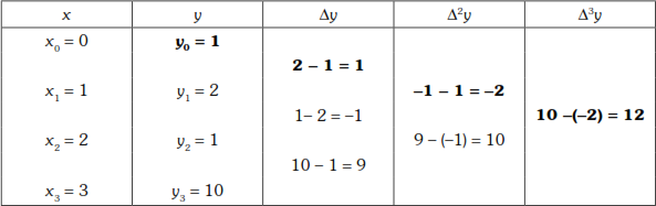
![]()

∴ ![]()
When x = 4,
![]()
Example 2
A third degree polynomial passes through the points (0, −1), (1, 1), (2, 1) and (3, –2). Using Newton’s forward formula, find the polynomial. Hence find the value at 1.5.
Solution
We use Newton’s forward formula to find the polynomial passing through (0, –1) (1, 1), (2, 1) and (3, –2).
Newton’s forward formula is
![]()
where
![]()
Here
![]() (1)
(1)
Now we form the forward difference table.

![]()
Substituting in (1), we get

Since u = x, the polynomial is ![]()

Example 3
The population of a city in Census taken once in 10 years is given below. Estimate the population in the year 1955.
| Year | 1951 | 1961 | 1971 | 1981 |
| Population in thousands | 35 | 42 | 58 | 84 |
Solution
Let us denote year as x, and population as y.
Let y = f(x)
x = 1955 is near the beginning of the table. So we use Newton’s forward difference formula to find y.
Newton’s forward formula is
![]() (1)
(1)
where ![]() . Here
. Here ![]()
![]()
When ![]()
Now we form the forward difference table.

∴ ![]()
and when x = 1955, u = 0.4
Substituting in (1), we get

Example 4
From the data given below find the number of students whose weight is between 60 to 70.
| Weight in lbs: | 0–40 | 40–60 | 60–80 | 80–100 | 100–120 |
| No. of students | 250 | 120 | 100 | 70 | 50 |
Solution
Let weight be denoted by x and number of students be denoted by y
Let y = f(x)
We use Newton’s forward formula to find y when x lies between 60–70.
We rewrite the table as cumulative table showing the number of students less than x lbs.
Newton’s forward formula is
 (1)
(1)
where ![]() .
.
Here ![]() ∴
∴ ![]()
We shall find y when x = 70
∴ ![]()
Now we form the forward table.
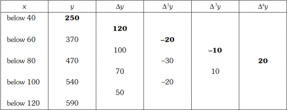
Hence ![]()
![]() and when
and when ![]()
Substituting in (1), we get

No. of students whose weight is below 70 is 424
∴ no. of students whose weight is between 60 – 70 is = 424 – 370 = 54
Example 5
If
| x | 0 | 1 | 2 | 3 | 4 | 5 |
| y | 27 | 32 | 25 | 36 | 32 | 41 |
then find approximately the value of y when x = −0.5.
Solution
Let y =f(x). To find y when x = –0.5.
x = –0.5 is outside the table value and is near the beginning of the table.
∴ It is extrapolation. So, we use Newton’s forward formula to find y when x = –0.5
Newton’s forward formula is
 (1)
(1)
where ![]() . Here
. Here ![]()
When ![]()
Now we form the difference table.

Hence ![]()
and when ![]()
Substituting in (1), we get

Example 6
The following table gives melting point of an alloy of zinc and lead, θ is the temperature and x is the percentage of lead. Using Newton’s interpolation formula find θ when x = 84.
| x | 40 | 50 | 60 | 70 | 80 | 90 |
| θ | 184 | 204 | 226 | 250 | 276 | 304 |
Solution
Let y = f(x), where y = θ,
x = 84 is near the end of the table.
∴ we use Newton’s backward formula to find θ when x = 84.
Newton’s backward formula is
 (1)
(1)
where ![]()
![]()
When
![]() ,
, ![]()
Now we form the table.

Hence ![]()
and when ![]()
Substituting in (1) we get

Example 7
If lx represents the number of people living at age x in a life table, find l47, given l20 = 512, l30 = 439, l40 = 346 and l50 = 243.
Solution
Let y = lx.
x = 47 is near the end of the table values. So, we use Newton’s backward formula to find l47.
Newton’s backward formula is
 (1)
(1)
where ![]() . Here
. Here ![]() ∴
∴ ![]()
When ![]()
Now we form the difference table.

∴ ![]()
and when x = 47, v = –0.3
Substituting in (1), we get

Hence the number of people expected to live at the age of 47 is 274.
Example 8
A function y is given by the following table. Estimate the value of y when x = 5.
| x | 0 | 1 | 2 | 3 | 4 |
| y | 79 | 91 | 105 | 116 | 127 |
Solution
Let y = f(x).
We want to find y when x = 5, which is outside the end of the table and hence extrapolation. So, we use Newton’s backward formula to find y when x = 5.
Newton’s backward formula is
 (1)
(1)
where ![]() . Here
. Here ![]() ∴
∴ ![]()
When ![]()
Now we form the difference table.
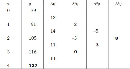
Here
![]()
![]() and when
and when ![]()
Substituting in (1), we get

Example 9
The following are data from the steam table.
| Temperature °C | 140 | 150 | 160 | 170 | 180 |
| Pressure kg/cm2 | 3.685 | 4.854 | 6.302 | 8.076 | 10.225 |
Find the pressure at temperature 142°C and 175°C.
Solution
Let temperature be x°C and pressure be y kg/cm2
Let y = f(x)
Since x = 142°C is near the beginning of the table, we use Newton’s forward formula to find y.
Newton’s forward formula is
 (1)
(1)
where ![]() . Here
. Here ![]() ∴
∴ ![]()
When ![]()
We now form the forward difference table.
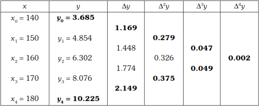
Here
![]()
When temperature is x = 142°C, then pressure

(ii) Since x = 175°C is near the end of the table, we use Newton’s backward formula.
Newton’s backward formula is
 (1)
(1)
where ![]()
When ![]()
From the difference table, we have
![]()

Example 10
Estimate the value of f(22) and f(42) from the following data:
| x | 20 | 25 | 30 | 35 | 40 | 45 |
| f (x) | 354 | 332 | 291 | 260 | 231 | 204 |
Solution
We find f(22) using Newton’s forward formula.
Newton’s forward formula is
 (1)
(1)
where ![]() . Here
. Here ![]() ∴
∴ ![]()
When ![]()
From forward difference table

![]()

To find y when ![]()
Given y = f(x)
x = 42 is near the end of the table. So, we use Newton’s backward formula to find f(42).
Newton’s backward formula is
 (1)
(1)
where ![]() . Here
. Here ![]()
![]()
When ![]()
![]()
and when x = 42, v = –0.6
Substituting in (1) we get

f(42) = 218.66 = 219 approximately
Exercises 4.2
- Use Newton’s backward formula to find a polynomial of degree 3 for the data f(–0.75) = –0.0781250, f(–0.5) = –0.024750, f(–0.25) = 0.33493750, f(0) = 1.10100. Hence find

- From the following table, find the value of tan 45° 15′
x0 45 46 47 48 49 50 tan x0 1.0 1.03553 1.07237 1.11061 1.15037 1.19175 - Find f(2.5) using Newton’s forward difference formula for the given data.
x 1 2 3 4 5 
0 1 8 27 64 - Using Newton’s backward difference formula find the area of a circle of diameter 98 from the given table of diameter and area of a circle.
Diameter 80 85 90 95 100 Area 5026 5674 6362 7088 7854 - Find
 given that
- (6) A function f(x) is given by the following table. Estimate f(0.2) by any appropriate formula.
x 0 1 2 3 4 5 6 f(x) 176 185 194 203 212 220 229 - Find the value of f(x) when x = 32, given the following table:
x 30 35 40 45 50 f(x) 15.9 14.9 14.1 13.3 12.5 - Find the number of students from the following data who secured marks not more than 45.
Marks 30–40 40–50 50–60 60–70 70–80 No of students 35 48 70 40 22 - The following are the annual premiums charge by the L.I.C of India for a policy of Rs. 1000. Calculate the premium payable at the age of 22.
Age in year 20 25 30 35 40 Premium Rs. 23 26 30 35 42 - Calculate the value of sin 33° 13′ 30″ from the following table of sines.
x° 30 31 32 33 34 sin x° 0.5000 0.5150 0.5290 0.5446 0.5592 - The table gives the distance in nautical miles of the visible horizon for the given height in feet above the earths surface. Find the values of y when x = 218′ and x = 410′.
x 100 150 200 250 300 350 400 y 10.63 13.03 15.04 16.81 18.42 19.90 21.27 - Find u6 given that
u0 u1 u2 u3 u4 u5 25 25 22 18 15 5 - By appropriate formula estimate the population for the year 2006, given
Year: 2001 2002 2003 2004 2005 Population in thousands: 251 279 319 383 483 - A function y is given by the following table. Estimate the value of y when x = 5.
x 0 1 2 3 4 y 79 91 105 116 127 - Two variables x and y have the following related values
x 0 10 20 30 40 50 60 y 2501 2795 2838 3030 3050 3381 3888 Find y when x = 54.
- Given
x 0.5 0.6 0.7 0.8 0.9 1.0 1.1 1.2 y = f(x) 0.34375 0.87616 1.47697 2.17408 3.00139 4 5.21941 6.71872 Find f(1.18).
Answers 4.2
- (1)
 ,
, 
- (2) 1.00876 (3) 3.4 (4) 7543 (5) –161
- (6) 177.67 (7) 15.45 (8) 51 (9) 24.04
- 0.54788 (11) 15.697, 21.53 (12) 20 (13) 631
- 149 (15) 3674.97 (16) 6.39328
4.3 CENTRAL DIFFERENCE INTERPOLATION FORMULAE
We have seen that Newton’s formward formula is suitable to interpolate near the beginning of a table of values and Newton’s backward formula is suitable to interpolate near the end of the table with equally spaced arguments.
For interpolating near the middle of the table the central difference formulae are better suited than others. The central difference formulae employ the difference lying as nearly as possible on a horizontal line through y0 near the centre.
We will discuss the following central difference formulae.
- Gauss’s forward formula
- Gauss’s backward formula
- Stirling’s formula
- Bessel’s formula
- Everett’s formula.
Of these Bessel’s and Stirlings are the most important ones.
Central difference table
Let ![]() be the function. Let
be the function. Let ![]() be the values of y corresponding to
be the values of y corresponding to ![]() and
and ![]() be the values corresponding to
be the values corresponding to ![]()
Then, the difference table with these values on either side of ![]() is given by the table below.
is given by the table below.
Put ![]() , where
, where ![]() is the origin.
is the origin.
The values of u corresponding to
![]()
are respectively
![]()


4.3.1 Gauss’s Forward Formula for Interpolation
Gauss’s forward Interpolation formula is
![]()
Proof: We derive Gauss’s forward difference interpolation formula from Newton’s forward formula and using even differences on the horizontal line through ![]() and odd differences on the horizontal line between
and odd differences on the horizontal line between ![]() and
and ![]() from the central difference table.
from the central difference table.
Newton’s forward formula is
![]() (1)
(1)
where ![]()
From the Central difference table, we have


Similarly,
![]()
![]()
Similarly, ![]() and so on.
and so on.
Substituting for ![]() in (1) we get
in (1) we get


If the symbol  , then the formula can be written as

Note:
- Gauss’s forward formula involves even differences on the central line and odd differences below the central line as

- Gauss’s forward formula is mainly used to interpolate if
 .
. - Since it is measured from the origin forwardly, this formula is called forward formula.
WORKED EXAMPLES
Example 1
Use Gauss’s forward formula to find the value of y when ![]() from the following table.
from the following table.
| x | 1.5 | 2 | 2.5 | 3 | 3.5 | 4 |
| y | 37.9 | 246.2 | 409.3 | 537.2 | 636.3 | 715.9 |
Solution
We use Gauss’s forward formula to find y when ![]() since it is near the middle of the given table.
since it is near the middle of the given table.
Gauss’s forward formula is
![]()
where ![]() and
and ![]() is the origin. Here
is the origin. Here ![]()
We take ![]() , since
, since ![]() lies is between
lies is between ![]() and
and ![]()
![]()
When x = 2.7, ![]()
We shall form the forward difference table.
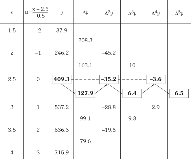

Substituting in (1), we get

When ![]()

When x = 2.7, y = 464.31
Example 2
Using Gauss’s forward formula find ![]() , given that
, given that
![]()
Solution
The given values of x are 21, 25, 29, 33, 37 and the corresponding y values are
![]()
![]() is near the middle of the table.
is near the middle of the table.
So, we use Gauss’s forward formula to find y when ![]() and formula is
and formula is
 (1)
(1)
where ![]() and
and ![]() is the origin.
is the origin.
Here ![]() and take
and take ![]() since
since ![]() lies between
lies between ![]() and
and ![]() .
.
![]()
When x = 30,
![]()
Now we shall form the central difference table.


Substituting in (1), we get

When ![]()


∴ ![]()
Example 3
Use Gauss’s forward interpolation formula to find log sin 0°16′8.5″ from the given table.
| x | 0°16′7″ | 0°16′8″ | 0°16′9″ | 0°16′10″ |
| 7.67100 | 7.67145 | 7.67190 | 7.67235 |
Solution
We use Gauss’s forward formula to find ![]() , since
, since ![]() is near the middle of the table.
is near the middle of the table.
Gauss’s forward formula is
![]() (1)
(1)
where ![]() and
and ![]() is the origin
is the origin
Here ![]() and take
and take ![]() , since
, since ![]() lies between
lies between ![]() and
and ![]() .
.
∴ ![]()
When ![]()
We shall form the central difference table.

![]()
Substituting in (1), we get
![]()
When ![]()
![]()
∴ loge sin 0° 16¢8.5′ = 7.671675
Example 4
Estimate the value of ![]() from the following data.
from the following data.
| x | 0 | 1 | 2 | 3 | 4 | 5 | 6 |
| 176 | 185 | 194 | 203 | 212 | 220 | 229 |
Solution
We use Gauss’s forward formula to find ![]() since
since ![]() is near the middle of the table.
is near the middle of the table.
Gauss’s forward formula is
 (2)
(2)
where ![]() and
and ![]() is the origin.
is the origin.
Here ![]() and take
and take ![]() , since
, since ![]() lies between
lies between ![]() and
and ![]() .
.
∴ ![]() .
.
When ![]() ,
, ![]()
We shall form the central difference table.


Substituting in (1), we get

When ![]()

Example 5
Interpolate by means of Gauss’s forward formula the value of ![]() given that
given that ![]()
Solution
The given values of the arguments x are 25, 30, 35, 40 and the corresponding values of y are ![]()
![]() is near the middle of the table.
is near the middle of the table.
So, we use Gauss’s forward formula to find ![]() .
.
Gauss’s forward formula is
 (1)
(1)
where ![]() and
and ![]() is the origin.
is the origin.
Here ![]() and take
and take ![]() , since
, since ![]() lies between
lies between ![]() and
and ![]() .
.
∴ ![]()
When
![]() ,
, ![]()
We shall form the central difference table.

![]()
Substituting in (1), we get
![]()
When ![]()

4.3.2 Gauss’s Backward Formula for Interpolation
Gauss’s Backward formula for Interpolation is
![]()
Proof: We derive Gauss’s backward difference formula from Newton’s forward formula by using even differences along the central line and odd differences above the central line.
Newton’s forward formula is
![]() (1)
(1)
where ![]() and x0 is the origin.
and x0 is the origin.
We have Δy0 – Δy–1 = Δ2y–1
⇒ Δy0 = Δy–1 + Δ2y–1
Similarly
Δ2y0 = Δ2y–1 + Δ3y–1
Δ3y0 = Δ3y–1 + Δ4y–1 and so on.
Also
Δ3y–1 -Δ3y–2 = Δ4y–2
⇒ Δ3y–1 = Δ3y–2 + Δ4y–2
Δ4y–1 = Δ4y–2 + Δ5y–2 and so on.
Substituting ![]() in (1) we get
in (1) we get


![]()


![]()
⇒ 
where 
Note:
- Gauss’s backward formula uses the differences on the indicated path

- Gauss’s backward formula is used for interpolation if
 .
.
Because of this reason, Gauss’s backward formula is some times known as Gauss’s formula for negative interpolation.
WORKED EXAMPLES
Example 1
Given that ![]()
![]()
![]()
![]() Show by Gauss’s backward formula
Show by Gauss’s backward formula ![]()
Solution
Given values of x are 12500, 12510, 12520, 12530.
Required the value of ![]() by Gauss’s backward formula.
by Gauss’s backward formula.
Let ![]() Then to find
Then to find ![]()
Gauss’s backward formula is
![]() (1)
(1)
where ![]() and
and ![]() is the origin.
is the origin.
Here ![]() and take
and take ![]() , since
, since ![]() lies between
lies between ![]() and
and ![]()
∴ ![]()
When ![]() ,
, ![]()
We shall form the central difference table.

![]()
Substituting in (1), we get

When ![]()


Example 2
Given the following data
| x | 1.72 | 1.73 | 1.74 | 1.75 | 1.76 |
| 0.17907 | 0.17728 | 0.17552 | 0.17377 | 0.17204 |
Find the value of ![]() using Gauss’s backward formula.
using Gauss’s backward formula.
Solution
Required the value of ![]() when
when ![]() by Gauss’s backward formula
by Gauss’s backward formula
 (1)
(1)
Where ![]() and
and ![]() is the origin.
is the origin.
Here ![]() and take
and take ![]() since
since ![]() lies between
lies between ![]() and
and ![]()
∴![]()
When ![]()
![]()
We shall form the central difference table.


Substituting in (1), we get

When ![]() we get
we get

∴ ![]()
Example 3
Using Gauss’s backward formula estimate the number of persons earnings wages between Rs. 60 and 70 from the following data.
| Wages (Rs.) | Below 40 | 40–60 | 60–80 | 80–100 | 100–120 |
| No of person’s (in thousands) | 250 | 120 | 100 | 70 | 50 |
Solution
We take the given intervals as 20–40, 40–60, 60–80, 80–100, 100–120.
Let the middle points of the intervals be the x-values and numbers of persons as the corrsponding y values.
| Values of x | 30 | 50 | 70 | 90 | 110 |
| y | 250 | 120 | 100 | 70 | 50 |
To find the number of persons earning wages between Rs. 60 and 70, we use Gauss’s backward formula.
Gauss’s backward formula is
![]() (1)
(1)
where ![]() and
and ![]() is the origin.
is the origin.
Here ![]()
For the interval 60–70, middle value is ![]()
∴ take ![]() , since
, since ![]() lies between
lies between ![]() and
and ![]()
∴ ![]()
When ![]() ,
,
![]()
We shall form the central difference table.

![]()
Substituting in (1), we get
![]()
When ![]() , we get
, we get

∴ the number of persons in the wage range 60 to 70 is equal to 104.
Exercises 4.3
- Using Gauss’s forward formula find
 given that
x 2 3 4 5 
2.426 3.454 4.784 6.986 - Given that
Year 1930 1932 1934 1936 1938 1940 Population (in thousand) 12 16 21 27 32 40 Using Newton-Gauss’s forward formula find the population of the town in 1935.
- Using Gauss forward formula find the value of y28.3 given that y26 = 0.038462,

- Given sin 25° 41′ 40″ = 0.433572, sin 25° 42′ 0′ = 0433659, sin 25° 42′ 20″ = 0.433746, sin 25° 42′ 40″ = 0.433834. Find the value of sin 25° 42′ 10″ by Gauss’s forward formula.
- If
 find
find  approximately.
 - Given
 , find the value of
  by Gauss’s backward formula.
 - The specific gravities of Zinc sulphate solutions of different concentrations at
 are given below
Concentration (%): 10 12 14 16 18 20 22 Specific gravity: 1.059 1.073 1.085 1.097 1.110 1.124 1.137 Find the specific gravity of 15.8% solution at
 , using Gauss’s Backward formula.
 - Interpolate by means of Gauss’s backward formula the sales of a concern for the year 1997 given that
Year: 1962 1972 1982 1992 2002 2012 Sales (in cores of Rs.) 12 15 20 27 39 52 - Find the value of
 by Gauss’s backward formula, given that
x: 


cos x: 0.6428 0.6293 0.6152 0.6018 0.5878
Answers 4.3
- 4.034 (2) 24.046875 (3) 0.0353355
- 0.43 3703 (5) 7.6 (6) 3165.36
- 1.0958 (8) 32.625 crores of Rs. (9) 0.6198
4.3.3. Stirling’s Formula for Interpolation
Stirling’s formula is

Proof: Stirling’s formula is derived by taking the average Gauss’s forward and backward formulae.
Gauss’s forward formula is
 (1)
(1)
Gauss’s backward formula is
 (2)
(2)
Adding (1) and (2), we get


This is called Stirling’s formula or Newton-Stirling’s formula.
Note:
- Stirling’s formula involves average of odd difference above and below the central line and even differences on the central line as shown.

- Stirling’s formula gives fairly accurate results when
 , though this formula can be used if
  .
.
WORKED EXAMPLES
Example 1
Given
| 0 | 0.0875 | 0.1763 | 0.2679 | 0.3640 | 0.4663 | 0.5774 |
Find the value of ![]() using Stirling’s formula.
using Stirling’s formula.
Solution
Let ![]()
Given ![]()
To find the value of ![]() .
.
We use Stirling’s formula to find y when x = 16
Stirling’s formula is

where ![]() and x0 is the origin.
and x0 is the origin.
Here ![]() and take
and take ![]() , since
, since ![]() lies between
lies between ![]() and
and ![]()
![]()
When ![]() ,
,
![]()
We shall form the central difference table.


Substituting in (1), we get

When ![]() , we get
, we get

Example 2
The following table gives the values of the probability integral ![]() Find the value o the integral when
Find the value o the integral when ![]() .
.
| x | 0.51 | 0.52 | 0.53 | 0.54 | 0.55 | 0.56 |
| 0.52924 | 0.53789 | 0.54646 | 0.55494 | 0.56332 | 0.57162 |
Solution
Required to find ![]() when
when ![]() by using Stirling’s formula.
by using Stirling’s formula.
Stirling’s formula is
 (1)
(1)
where ![]() and
and ![]() is the origin.
is the origin.
Here ![]() and take
and take ![]() , since
, since ![]() lies between
lies between ![]() and
and ![]()
∴ ![]()
When ![]()
![]()
We shall form the central difference table.


Substituting in (1), we get

When ![]() , we get
, we get

when ![]()
Example 3
Using Stirling’s formula find the annual net premium at the age of 25 from the table of annual net premium given below.
| Age | 20 | 24 | 28 | 32 |
| Premium | 0.01427 | 0.01581 | 0.01772 | 0.01996 |
Solution
Let us denote age by x and premium as y.
Required, the net premium at the age of 25 using Stirling’s formula.
That is to find y when x = 25.
Stirling’s formula is
![]() (1)
(1)
where ![]() and
and ![]() is the origin.
is the origin.
Here ![]() and take
and take ![]() since
since ![]() lies between
lies between ![]() and
and ![]()
∴ ![]()
When ![]()
![]()
We shall form the central difference table.

Here h = 4 and take x0 = 24, since x = 25 lies between x = 24 and x = 28
![]()
Substituting in (1), we get

When ![]()

∴ net Premium when ![]() is 0.01625
is 0.01625
Example 4
Find the value of ![]() and
and ![]() from the following table using Stirling’s formula.
from the following table using Stirling’s formula.
| x | 1.50 | 1.60 | 1.70 | 1.80 | 1.90 |
| 17.609 | 20.412 | 23.045 | 25.527 | 27.875 |
Solution
Let ![]()
Required the values of y when ![]() and
and ![]() by using Stirling’s formula.
by using Stirling’s formula.
Stirling’s formula is
 (1)
(1)
where ![]() and
and ![]() is the origin.
is the origin.
Here ![]() and take the orgin as
and take the orgin as ![]() since x = 1.63 lies between 1.60 and 1.70
since x = 1.63 lies between 1.60 and 1.70
∴ ![]()
When ![]()
![]()
We shall form the central difference table when ![]()

![]()
Substituting in (1), we get

When ![]()
![]()
We use Stirlings formula if ![]() only. So we cannot take the origin as x = 1.60 to find y when x = 1.67, since
only. So we cannot take the origin as x = 1.60 to find y when x = 1.67, since ![]()
So, we change the origin to x = 1.70, to find y when x = 1.67
∴ ![]()
When ![]()
![]() [
[![]() lies is the interval
lies is the interval ![]() ]
]
When ![]() the difference table is
the difference table is


Substituting in (1), we get
![]()

4.3.4 Bessel’s Formula for Interpolation
Bessel’s formula is

Proof: We derive the Bessel’s formula using Gauss’s forward and backward formula.
Gauss’s forward formula is
 (1)
(1)
Gauss’s backward formula is
 (2)
(2)
Shifting the origin of u from 0 to 1, that is replace u by ![]() in backward formula, we get
in backward formula, we get
![]()
![]() (3)
(3)
Adding (1) and (3) we get


This is Bessel’s formula.
If we put ![]() then
then ![]() and Bessel’s formula reduces to a more symmetrical form.
and Bessel’s formula reduces to a more symmetrical form.

Note:
- Bessel’s formula employs odd differences below the central line and the means of even differences on and below the central line.
- If
 Bessel’s formula is preferable. However it will give more accurate result when interpolating near the middle of the interval
When
 Bessel’s formula gives best results with minimum number of terms.
 - When
 we get the special case of Bessel’s formula.

This is called formula for interpolating to halves.
WORKED EXAMPLES
Example 1
Apply Bessel’s formula to find log103375, given log10310 = 2.49137, log10320 = 2.250515, log10330 = 2.51851, log10340 = 2.53148, log10350 = 2.54407, log10360 = 2.55630.
Solution
Required the value of ![]() using Bessel’s formula,
using Bessel’s formula,
Bessel’s formula is
 (1)
(1)
where ![]() and
and ![]() is the origin.
is the origin.
The given function is ![]() and the x values are 310, 320, 330, 340, 350, 360.
and the x values are 310, 320, 330, 340, 350, 360.

Here ![]() and take the origin as
and take the origin as ![]() , since
, since ![]() lies between
lies between ![]() and
and ![]()
∴ ![]()
When ![]()
![]()
We shall form the difference table.


Substituting in (1), we get


Example 2
The area A of a circle and diameter d is given by the following table.
| d | 80 | 85 | 90 | 95 | 100 |
| Area A | 5026 | 5674 | 6362 | 7088 | 7854 |
Find the area when the diameter is 91.
Solution
Let us denote the diameter d as x and area A as y.
Required, the area y when x = 91.
We use Bessel’s formula.
Bessel’s formula is
 (1)
(1)
where ![]() and
and ![]() is the origin.
is the origin.
Here ![]() and take the origin as
and take the origin as ![]() since
since ![]() lies between
lies between ![]() and
and ![]()
∴ ![]()
When ![]()
![]()
We shall form the central difference table.


Substituting in (1), we get

∴ area = 6504.1248 sq. unit
Example 3
Given ![]() and fifth differences are constant.
and fifth differences are constant.
Prove that 
Where ![]()
Solution
Given the values ![]() are such that the fifth differences are constant.
are such that the fifth differences are constant.
∴ 6th, 7th … differences are zero.
![]() (1)
(1)
Bessel’s formula for ![]() is
is
![]()
Now shift the origin to 2, then ![]() and so on.
and so on.
∴ ![]()
But

Similarly,
![]()

Example 4
Using Bessel’s interpolation formula show that ![]() assuming suitable level of approximation.
assuming suitable level of approximation.
Solution
Bessels formula is
 (1)
(1)
Replacing u by x in (1) we get

Assuming the fourth order and higher differences are very small, neglecting them and putting ![]() we get
we get

Now shifting the origin to x,
![]()
4.3.5 Laplace-Everett Formula for Interpolation
Laplace-Everett’s formula for interpolation is

where v = 1−u.
Proof: Laplace-Everett’s formula is obtained from Gauss’s forward formula by replacing the odd differences interms of even differences
Gauss forward formula is
 (1)
(1)
Now ![]()
Substituting in (1), we get


This formula is usually written in a more convenient form by putting ![]() in the terms with negative sign.
in the terms with negative sign.


where ![]()
Note:
- This formula involves the even differences on and below the central line.
- This formula is used when u lies between 0 and 1, but more accurate results will be obtained when
 or when
  or vice-versa.
WORKED EXAMPLES
Example 1
From the following table find ![]() using Everett’s formula.
using Everett’s formula.
| x | 20 | 25 | 30 | 35 | 40 |
| 11.4699 | 12.7834 | 13.7648 | 14.4982 | 15.0463 |
Solution
Everett’s formula is
 (1)
(1)
where ![]() and
and ![]() and
and ![]() is the origin.
is the origin.
Here ![]() and take
and take ![]() , since
, since ![]() lies between
lies between ![]() and
and ![]() .
.
∴ ![]()
When x = 34,

We shall form the difference table.


Substituting in (1), we get

∴ when ![]()
Example 2
Apply Everett’s formula to obtain ![]() given
given ![]()
![]()
Solution
Everett’s formula is

where ![]() ,
, ![]() and
and ![]() is the origin.
is the origin.
The given values of x are 20, 24, 28, 32.
Required the value of y when x = 25
Here ![]() and take
and take ![]() since
since ![]() lies between
lies between ![]() and
and ![]()

We shall form the difference table.


Substituting in (1), we get

∴ when ![]()
Example 3
If the third differences of ![]() are constant, show that
are constant, show that

where ![]()
Solution
We shall prove the result using Everett’s formula.
Since the third differences are constants the fourth and higher differences are zero.
Everett’s formula is
![]()
where ![]() , and
, and ![]() .
.
Here ![]()
∴ the formula becomes
![]()
Exercises 4.4
- Using Stirlings formula find
 given
given
x 1 1.1 1.2 1.3 1.4 
0.841 0.891 0.932 0.963 0.985 - Using Sitrling’s formula find
 given
given
x 1 6 11 16 21 
831 723 592 430 392 - Using Stirling’s formula find
 given
given  , where
  represents the number of persons at age x years in a life table.
 - Using Stirling’s formula find the value
 given that
x 1.01 1.015 1.02 1.025 1.03 
1.64463 2.10524 2.69159 3.43711 4.38391 - (5) Apply Stirling’s formula to find the value of
 given that
x 3.4 4.4 5.4 6.4 7.4 8.4 
1156 1936 2916 4096 5476 7056 - (6) Using Bessel’s formula to find the value of y when x = 15, given that
x 10 12 14 16 18 20 y 51.21 60.24 75.32 96.02 119.78 151.45 - (7) Using Bessel’s formula find
 given
given
x 15 20 25 30 35 40 
10.3797 12.4622 14.0939 15.3725 16.3742 17.1591 - (8) Use Bessel’s formula to obtain
 given
given 
- (9) Given
x 20 24 28 32 
24 32 35 40 Find
 using Bessel’s formula.
 - If
x 30 35 40 45 50 55 60 
771 862 1001 1224 1572 2123 2983 then find
 by Everett’s method.
 - Use Everett’s formula to obtain
 given that

Answers 4.4
- 0.934 (2) 673.58 (3) 395 (4) 2.86155
- 2959.36 (6) 85.189 (7) 15.0818 (8) 3250.8715
- 32.945 (10) 1431.5 (11) 1.073
4.4 INTERPolatiON WITH UNEQUAL INTERVALS
Newton’s forward and backward formulae can be applied when the arguments are equally spaced. When the arguments are unequally spaced, we use Lagrange’s interpolation formula.
4.4.1 Lagrange’s Interpolation Formula
Theorem 4.2
Let ![]() be the entries corresponding to the arguments
be the entries corresponding to the arguments ![]() which are not necessarily equally spaced, then Lagrange’s interpolation formula is
which are not necessarily equally spaced, then Lagrange’s interpolation formula is

Proof: Let ![]() be the entries corresponding to the arguments
be the entries corresponding to the arguments ![]() not necessarily equally spaced, then the interpolating polynomial
not necessarily equally spaced, then the interpolating polynomial ![]() for
for ![]() is of degree n and let
is of degree n and let

where ![]() are constants to be determined such that
are constants to be determined such that
![]()
When ![]()

When ![]()

Similarly, when ![]() we get
we get

 (1)
(1)
In the place of ![]() we can write
we can write ![]()

WORKED EXAMPLES
Example 1
Find f(x) as a polynomial in x from the given data and find f(8).
| x | 3 | 7 | 9 | 10 |
| f(x) | 168 | 120 | 172 | 63 |
Solution
Given the values of x and y are
![]() and
and ![]()
The values of x are not equally spaced. So we use Lagrange’s formula to find y = f(x)
Lagrange’s formula for a set of four pairs of values is


Note: ![]()
Example 2
Find the polynomial f(x) by using Lagrange’s formula and hence find f(3) for the following values of x and y.
| x | 0 | 1 | 2 | 5 |
| y | 2 | 3 | 12 | 147 |
and hence find f(3).
Solution
![]()
The values of x are not equally spaced so we use Lagrange’s formula to find y = f(x)
Lagrange’s formula for a set of four pairs of values is


Example 3
Using Lagrange’s formula prove that
![]()
Solution
From the given equation, the values of x involved are ![]() and the corresponding y values are
and the corresponding y values are ![]()
The values of x are not equally spaced.
So, we use Lagrange’s formula to find y = f(x)
Lagrange’s formula for a set of four pairs of values is

When x = 1, we get

Example 4
Given the values
| x | 5 | 7 | 11 | 13 | 17 |
| y = x f(x) | 150 | 392 | 1452 | 2366 | 5202 |
Evaluate f(9) using Lagrange’s formula.
Solution
Given the values of x and y are
![]()
The values of x are not equally spaced, so we use Lagrange’s formula to find y = f(x).
Lagrange’s formula for a set of five pairs of values is


When x = 9,


Exercises 4.5
- Using Lagrange’s formula fit a polynomial to the data and find f(5).
x –1 1 2 f(x) 7 5 15 - Using Lagrange’s formula find y (10) given that y (5) = 12, y (6) = 13, y (9) = 14, y (11) = 16.
- Using Lagrange’s interpolation formula calculate the profit in the year 2000 from the following data:
Year 1997 1999 2001 2002 Profit in Lakhs Rs. 43 65 159 248 - Apply Lagrange’s formula to find f(5) and f(6) given that f(l) = 2, f(2) = 4, f(3) = 8, f(4) = 16, and f(7) = 128
- Find the form of the function ux given that

- Use Lagrange’s formula to find f(5) from the following data:
x 2 3 4 6 7 f(x) 1 5 13 61 125 - Find the form of ux, give that


- Find u5 given that u1 = 4, u2 = 7, u4 = 13 and u7 = 30
- The following table gives the premium payable at the ages in years completed. Interpolate the premium payable at the age of 35 completed.
Age completed in years: 25 30 40 60 Premium in Rs. 50 55 70 95 - From the following table find the value of y when x = 10
x 5 6 9 11 y 12 13 14 16
Answers 4.5
 (2)
(2) 
 (4)
(4) 
 (6)
(6) 
 (8)
(8) 
 (10)
(10) 
4.4.2 Divided Differences
In forward and backward differences for equally spaced arguments we considered only differences of the entries. But in divided differences, we divide this difference by difference of the corresponding arguments.
Let a function y = f(x) take values ![]() corresponding to the arguments
corresponding to the arguments ![]() , not necessarily equally spaced.
, not necessarily equally spaced.
The first divided difference for the arguments x0, x1 is defined as ![]() .
.
It is denoted by ![]()
We shall denote,
![]()
Similarly,

The second divided difference for the arguments ![]() is defined as
is defined as

The second difference for ![]() is
is

The third divided difference for ![]() is
is

The third difference for ![]() is
is
 and so on.
Properties of divided differences
- 1. The divided differences are symmetric functions of their arguments.
For example

- 2. The nth divided differences of a polynomial of degree n are constants.
- 3.

and
 is constant.
 This shows that Δ is a linear operator.
- 4. The nth divided difference is a quotient of two determinants, each of order n + 1.
We have

 is a quotient of two determinant of same order 2.
Similarly we can write the other divided differences as a quotient of determinants of the same order.
WORKED EXAMPLES
Example 1
For the function ![]() , prove that the third divided difference with arguments a, b, c, d is equal to
, prove that the third divided difference with arguments a, b, c, d is equal to ![]()
Solution
Given

Similarly
![]()
Now

Similarly

Example 2
Prove that ![]()
Solution
Given the function f(x) = x3 and the arguments are x, y, z
∴ 
Similarly,
![]()
Now

Divided difference table
A divided difference table can be constructed using same principle as for ordinary difference tables. It is a diagonal difference table as illustrated by the following example.

4.4.3 Newton’s General Interpolation Formula or Newton’s Divided Difference Formula for Interpolation
Let ![]() be the given values of the function f(x) corresponding to unequally spaced arguments
be the given values of the function f(x) corresponding to unequally spaced arguments ![]() .
.
Newton’s general interpolation formula is

Proof: Corresponding to the given unequally arguments ![]() the values of the function f(x) are
the values of the function f(x) are ![]()
Let x be the argument for which the value is required.
Then for the arguments x0, x
 (1)
(1)
Again for the arguments x0, x1, x

Substituting in (1), we get
 (2)
(2)
Now for the arguments x0, x1, x2, x

Substituting in (2) we get,
 (3)
(3)
Proceeding in this way we obtain

where ![]() is the remainder term.
is the remainder term.
![]()
Let the interpolating polynomial be ![]()
If we put

then ![]()
We see that ![]() because
because ![]()
Hence the interpolation formula is ![]() or
or

Note: Using the relation between divided differences and ordinary differences from the general formula, we can deduce Newton’s forward and backward difference formulae for interpolation.
WORKED EXAMPLES
Example 1
Construct the divided difference table for the following data and find the value of f(2).
| x | 4 | 5 | 7 | 10 | 11 | 12 |
| f(x) | 50 | 102 | 296 | 800 | 1010 | 1224 |
Solution
Given value of x are ![]()
The values of x are unequally spaced, so we use Newton’s divided difference formula to find f(x) when x = 2.
Newton’s divided difference formula is
 (1)
(1)
We form the divided difference table.

(1) becomes

when x = 2,

Example 2
By using Newton’s divided difference formula find f(8), given
| x | 4 | 5 | 7 | 10 | 11 | 13 |
| f(x) | 48 | 100 | 294 | 900 | 1210 | 2028 |
Also find f(6), f(9), f(15).
Solution
Given the values of x are ![]()
The values of x are unequally spaced, so, we use Newton’s divided difference formula to find f(x) when x = 8.
Newton’s divided difference formula is
 (1)
(1)
We form the divided difference table.

(1) becomes

![]()
![]()
![]()
When x = 15
![]()
Example 3
Given the data
| x | 0 | 1 | 2 | 5 |
| f(x) | 2 | 3 | 12 | 147 |
Find the cubic function of x, using Newton’s divided difference formula, and hence find f(2).
Solution
Given ![]()
The values of x are unequally spaced. We use Newton’s divided difference formula to find f(x)
Newton’s divided difference formula is
 (1)
(1)
We form the divided difference table

∴ (1) becomes

When ![]()
Example 4
Find the third divided difference with arguments 2, 4, 9, 10 of the function f(x) = x3 – 2x.
Solution
Given the values of x are ![]()
and ![]()

We form the divided difference table to find the divided differences.

The third divided difference is Δ3f(x) = 1
Example 5
Given the following data, find f(x ) as a polynomial in x.
| x | 0 | 2 | 3 | 4 | 7 | 9 |
| f (x) | 4 | 26 | 58 | 112 | 466 | 922 |
Solution
Given ![]()
The values of x are unequally spaced. So, we find f(x) using Newton’s divided difference formula.
 (1)
(1)
We form the divided difference table

∴ (1) becomes
![]()
[∴ all higher powers are zero ]

Example 6
If f(0) = 0, f(l) = 0, f(2) = –12, f(4) = 0, f(5) = 600, f(7) = 7308, find a polynomial that satisfies this data using Newton’s divided difference formula. Hence find f(6).
Solution
Given the values of f(x) are
![]()
The values of x are unequally spaced. We use Newton’s divided difference formula to find f(x).
We form the divided difference table

∴ Newton’s divided difference formula is
 (1)
(1)
 when
when
![]()
Aliter:
![]()
Since 6 values of f(x) are given, f(x) is polynomial of degree 5.
Since f(0) = 0, f(1) = 0, f(4) = 9,
f(x) = 0 when x = 1 and x = 4.
So, by factor theorem ![]() are factors of f(x).
are factors of f(x).
![]() , where g(x) is a polynomial of degree 2.
, where g(x) is a polynomial of degree 2.
We shall find this polynomial g(x) by using the other three values
![]() .
.
When ![]()
When ![]()
When ![]()
We shall find g(x) by using Newton’s divided difference formula

By Newton’s divided difference formula

∴ the polynomial ![]()
Now
![]()
Exercises 4.6
- Given the following data:
x 3 7 9 10 f(x ) 168 120 72 63 Calculate f(6).
- Using Newton’s divided difference formula, find u(3) given


- Find f(10) using Newton’s divided difference formula given that
x 11 17 21 23 f(x ) 14646 83526 194486 279845 - Find the function f(x) from the following table:
x 0 1 4 5 f (x ) 8 11 78 123 - Given
 and log10 661 = 2.8202, find by divided difference the value of
- Find the equation of the curve passing through the points (–1, –21), (1, 15), (2, 12), (3, 3). Find also f(0).
- Find the cubic function from the following table:
x 0 1 3 4 f (x ) 1 4 40 85 - Given
 , find y2 using Newton’s divided difference formula.
Answers 4.6
- 147 (2) 100 (3) 130198
 (5) 2.8168 (6)
- f(x) = x3 + x2 + x + 1 (8) y2 = 4
4.5 ERRORS IN INTERPOLATION FORMULAE
We state some results without proof
- 1. Rolle’s Theorem: If the real function f is (i) Continuous on the closed interval [a, b] (ii) differentiable in the open interval (a, b) and (iii)
 then there exists at least one point c in (a, b) such that f’
Corollary: If
 is a polynomial of degree n and if
  then there is at least one
  such that
From this it follows that between two roots of
 there is a root of
In other words, the real roots of
 separate the real roots of the equation
More generally, if
 is a polynomial of degree n with a and b as the smallest and largest roots of
  then
then has (n –1) roots in (a, b)
 has (n –2) roots in (a, b)
 has at least one root in (a, b).
4.5.1 Remainder Term in Interpolation Formulae
Let ![]() be a function defined at
be a function defined at ![]() points
points ![]() and let
and let ![]() be continuous and it has continuous derivatives of all orders.
be continuous and it has continuous derivatives of all orders.
Let ![]() be a polynomial of degree not exceeding n such that
be a polynomial of degree not exceeding n such that ![]() i = 0, 1, 2, … , n, be an approximation for
i = 0, 1, 2, … , n, be an approximation for ![]()
Let ![]() (1)
(1)
Since ![]() for i = 0, 1, 2, … , n, we get
for i = 0, 1, 2, … , n, we get
![]()
⇒ g(xi) = 0, i = 0, 1, 2, …, n
∴ ![]() are roots of
are roots of ![]()
Hence
![]()
⇒ ![]() where
where ![]() is to be determined.
is to be determined.
∴ ![]() (2)
(2)
Now consider the function
![]() (3)
(3)
∴ ![]() for
for ![]()
Since ![]() and
and
![]() for i = 0, 1, 2, …,n and
for i = 0, 1, 2, …,n and ![]() for t = x by (2).
for t = x by (2).
Hence we find ![]() at n + 2 points
at n + 2 points ![]()
Also ![]() is continuous and differentiable n times in
is continuous and differentiable n times in ![]() where x0 is the least root and
where x0 is the least root and ![]() is the largest root.
is the largest root.
So, by Rolle’s theorem,
![]() has at least (n + 1) roots in
has at least (n + 1) roots in ![]()
![]() has at least n roots in
has at least n roots in ![]()
![]()
![]() has at least one root, say
has at least one root, say ![]() in
in ![]()
ie ![]()
But ![]()
Since ![]() is a polynomial of degree n,
is a polynomial of degree n, ![]()
Since ![]() we get
we get ![]()
⇒ ![]()
∴ ![]()
⇒ ![]()
Since ![]() is difference between the given function and the polynomial at any point x, it represents the error comitted in approximating the given function
is difference between the given function and the polynomial at any point x, it represents the error comitted in approximating the given function ![]() by the polynomial p(x)
by the polynomial p(x)
Hence the error = Rn
![]()
![]()
This error ![]() is called the truncation error for
is called the truncation error for ![]()
Remainder term in Newton’s forward formula
Let ![]() be equally spaced arguments with interval h.
be equally spaced arguments with interval h.
Then
![]()
∴ ![]()
and
![]()
∴ ![]()
![]()
Suppose the analytical form of ![]() is not known, then we cannot find the derivative
is not known, then we cannot find the derivative ![]()
∴ we replace ![]() by difference,
by difference,
we have the formula
![]()
⇒ ![]()
Put ![]()
∴ ![]()
Take ![]() then
then
![]()
∴ ![]()
∴ ![]()
Similarly we can find the error or remainder term in all the interpolation formulae.
We shall list them.
- Newton’s forward formula
- (a)

- (b)
 where
where 
- (a)
- Newton’s backward formula
- (a)

- (b)
 where
where 
- (a)
- Stirling’s formula
- (a)


- (a)
- Bessells formula in terms of v
- (a)

- (b)

- (a)
- Lagrange’s formula

WORKED EXAMPLES
Example 1
Find the error in the computation of sin 52° by using Newton’s forward formula, given that
| x | 45° | 50° | 55° | 60° |
| y = sin x | 0.7071 | 0.7660 | 0.8192 | 0.8660 |
Solution
The error in Newton’s forward formula is
![]()
where
![]()
We form the difference table.

Here ![]() (highest difference is third order)
(highest difference is third order)
∴ ![]()
When x = 52,
![]()
∴ ![]()
⇒ ![]()
Example 2
The values of ![]() for certain equidistant values of x are given below
for certain equidistant values of x are given below
| x | 1.72 | 1.73 | 1.74 | 1.75 | 1.76 |
| 0.1791 | 0.1773 | 0.1755 | 0.1738 | 0.1720 |
Find the error in computing ![]() by Stirling formula.
by Stirling formula.
Solution
The error in Stirling’s formula is
![]()
where ![]() x0 is the origin. Here x0 = 1.73, h = 0.01
x0 is the origin. Here x0 = 1.73, h = 0.01
When x = 1.735,
![]()

Here ![]()
∴ ![]()
![]()
Example 3
The following table gives certain values of ![]() Using Lagrange’s interpolation formula find the value of log 323.5. Also find the error.
Using Lagrange’s interpolation formula find the value of log 323.5. Also find the error.
| x | 321 | 322.8 | 324.2 | 325 |
| 2.50651 | 2.50893 | 2.51081 | 2.51188 |
Solution
The given values of x are x0 = 321, x1 = 322.8, x2 = 324.2, x3 = 325
Using Lagrange’s formula, it can be seen that log 323.5 = 2.50987
We shall now compute the error.
![]()
Here ![]()
∴ ![]()

But
![]()
![]()
 (Taking t0 = 321)
![]()

This shows that the error is less than 1 in the 11th place.
4.6 INTERPOLATION WITH A CUBIC SPLINE
4.6.0 Introduction
The interpolation formulae we have seen so far represent a single polynomial passing through the points (or nodes) in a given interval. If the number of points is more, then the interpolating polynomial for many functions will be of higher degree, which tend to oscillate more and more between nodes as the degree increases. Hence the values computed using these interpolating polynomials will be very rough, except the case where the given set of points is for a polynomial function. This drawback is overcome by the method of splines which was introduced by I.J. Schoenberg in 1946.
Instead of using a single high-degree interpolating polynomial in an interval ![]() we subdivide the interval into a number of subintervals and in each subinterval we use a lower degree polynomial and join them together to get an interpolating function, called spline. Thus spline interpolation is a piece wise polynomial interpolation. Though splines can be of any degree, cubic splines are the most popular ones. The name ‘spline is borrowed from the draftman’s spline, a device which is an elastic rod used for drawing a smooth curve through a set of points.
we subdivide the interval into a number of subintervals and in each subinterval we use a lower degree polynomial and join them together to get an interpolating function, called spline. Thus spline interpolation is a piece wise polynomial interpolation. Though splines can be of any degree, cubic splines are the most popular ones. The name ‘spline is borrowed from the draftman’s spline, a device which is an elastic rod used for drawing a smooth curve through a set of points.
4.6.1 Cubic Spline Interpolation
Let y = f(x) be the given function on the interval ![]()
Divide [a, b] into n subintervals by the points ![]()
where ![]()
Let S (x) be the cubic spline that approximates f(x) such that
- (i)
 for
for 
 is a third degree polynomial in each subinterval
 and
and  are continuous on (a, b)
ie. ![]()
ie. at the joining point xi, the successive cubics have the same slope and same curvature.
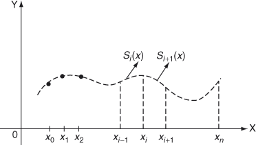
In each interval ![]() is a cubic polynomial, and so
is a cubic polynomial, and so ![]() is linear. By Lagrange’s formula, for the arguments
is linear. By Lagrange’s formula, for the arguments ![]() we have
we have
![]()
Since
![]() and
and ![]() and
and ![]()
![]()
Let
![]() and
and ![]()
∴ ![]()
Integrating twice w.r.to x, we get
 (2)
(2)
where c1 and c2 are arbitrary constants.
To find c1 and c2 use the hypothesis ![]() and
and ![]()
Put ![]() in (2)
in (2)
 (3)
(3)
Put ![]() in (2)
in (2)
 (4)
(4)

Subtracting, we get


where ![]() and
and ![]() are unknown quantities to be determined by using the continuity of
are unknown quantities to be determined by using the continuity of ![]() at the point
at the point ![]()
⇒ ![]()
ie. the left and right limits at ![]() are equal.
are equal.
Now differentiating (5) w.r.to x, we get
 (6)
(6)
Replacing i by i + 1, we get
![]() (7)
(7)
From (6),
 (8)
(8)
From (7),
 (9)
(9)
Since ![]()
we get from (8) and (9), (putting ![]() in the RHS)
in the RHS)
 (10)
(10)
This is true for all ![]()
Equations (10) give a system of (n – 1) linear equations in n + 1 unknowns ![]()
To solve for these unknowns we need two more equations. These two conditions may be taken in different ways.
We usually assume that outside the interval ![]() is flat or a straight line, then
is flat or a straight line, then ![]()
∴ ![]()
Thus we can solve for ![]() and these values are substituted in (5) to get the cubic spline
and these values are substituted in (5) to get the cubic spline ![]()
Note:
- The end conditions
 are called natural conditions because they yield a natural spline. It is called a natural spline because the draftman’s spline behaves like this.
 - Functions with abrupt local changes can be better approximated by cubic splines.
Working Rule: Given the table of values for y = f(x)
| x | x0 | x1 | … | xn |
| y | y0 | y1 | … | yn |
The cubic spline approximation S(x) for these points is ![]() in the interval
in the interval ![]() is
is

where ![]() and
and ![]()
WORKED EXAMPLES
Example 1
Obtain the cubic spline approximation for the function y = f(x) from the following data, given that ![]()
| x | –1 | 0 | 1 | 2 |
| y | –1 | 1 | 3 | 35 |
Solution
The given values of x and y are
x0 = -1, x1 = 0, x2 = 1, x3 = 2
and
y0 = -1, y1 = 1, y2 = 3, y3 = 35
The values of x are equally spaced with h = 1. Here n = 3.
The cubic spline for the interval ![]()
 (1)
(1)
where ![]()
![]() (2)
(2)
Given ![]() and
and ![]()
Put i = 1 in (2), we get,

Put i = 2 in (2), we get,

The cubic spline for ![]() is
is
 (3)
(3)
Put i = 1 in (1), then the interval ![]() is
is ![]()
Then the cubic spline for ![]() is
is

Put i = 2 in (1), then the interval ![]() is
is ![]()
Then the cubic spline for ![]() is
is


Put i = 3 in (1), then the interval ![]() is
is ![]()
Then the cubic spline for ![]() is
is

∴ the cubic spline approximation for the given function is

Example 2
Find the cubic spline approximation for the function f(x) given by the data:
| x | 0 | 1 | 2 | 3 |
| f(x) | 1 | 2 | 33 | 244 |
With ![]() . Hence estimate the value of f(2.5), f(1.5).
. Hence estimate the value of f(2.5), f(1.5).
Solution
Let y = f(x)
The given the values of x and y are
x0 = 0 , x1 = 1 , x2 = 2 , x3 = 3
y0 = 1 , y1 = 2 , y2 = 33 , y3 = 244
The values of x are equally spaced with h = 1, Here n = 3.
The cubic spline for the interval ![]() is
is

 (1)
(1)
where ![]() (2)
(2)
and ![]()
Put i = 1 in (2),

Put i = 2 in (2),

Solving we get ![]()
Put i = 1 in (1), then the interval ![]() is
is ![]()
Then the cubic spline for the interval ![]() is
is

Put i = 2 in (1), then the interval ![]() is
is ![]()
Then the cubic spline for the interval ![]() is
is


Put i = 3 in (1), then the interval ![]() is
is ![]()
Then the cubic spline for ![]() is
is

∴ the cubic spline is

When x = 2.5,
![]()
When x = 1.5,
![]()
Example 3
The following values of x an y are given
| x | 1 | 2 | 3 | 4 |
| y | 1 | 2 | 5 | 11 |
Find the cubic splines and evaluate y(1.5) and y′(3).
Solution
Given the values of x and y are
x0 = 1, x1 = 2, x2 = 3, x3 = 4
y0 = 1, y1 = 2, y3 = 5, y3 = 11
The values of x are equally spaced with h = 1. Here n = 3
The cubic spline for the interval ![]() is
is
 (1)
(1)
where
![]() (2)
(2)
We assume the conditions of natural spline ![]()
Putting i = 1 in (2) we get,
 (3)
(3)
Putting i = 2 in (2) we get,
 (4)
(4)
Solving (3) and (4), we get ![]()
Now Putting i = 1 in (1), then the interval ![]() is
is ![]() .
.
Then the cubic spline for the interval ![]() is
is


Putting i = 2 in (1), then the interval ![]() is
is ![]()
Then the cubic spline for the interval ![]() is
is

Putting i = 3 in (1), then the interval ![]() is
is ![]()
Then the cubic spline for ![]() is
is

∴ the cubic spline is

When x = 1.5,
![]()
Differentiating S(x) w.r.to x, we get

The derivates at the joining points should exist for the spline.
![]() can be obtained from [2, 3] or [3, 4] and they should be equal.
can be obtained from [2, 3] or [3, 4] and they should be equal.
So we can find from [2, 3], ![]()
Note:
If we find from [3, 4], ![]()
Exercises 4.7
- Given the following table, find f(2.5) using cubic spline functions.
i 0 1 2 3 xi 1 2 3 4 f(xi) 


- Find a natural cubic spline to the data, given
x: 1 2 3 4 y: 1 5 11 8 Hence find y(1.5) and y′(2).
- Find the natural cubic spline valid for the interval [3, 4] for the data
x: 1 2 3 4 y: 3 10 29 65 and hence find the value of y(3.2).
- Find the natural cubic spline for the data
x 0 2 4 6 f(x) 4 0 4 80 - Find the cubic spline interpolation for the data
x: 0 2 4 6 f(x): 1 9 41 41 Given

Answers 4.7


Short Answer Questions
- When Newton’s forward interpolation formula is used ?
- When Newton’s backward formula for interpolation is used ?
- State Newton’s backward formula for interpolation.
- State Newton’s forward formula for interpolation.
- What do you mean by interpolation?
- Given
 , find the value of u2.
 - A third degree polynomial passes through (0, –1), (1, 1), (2, 1) and (3, –2). Find its value at x = 4.
- Given f(0) = –1, f(1) = 1 and f(2) = 4, find the root of the Newton’s interpolating polynomial equation f(x) = 0.
- Form the divided difference table for the following data:
x 2 5 10 y 5 29 109 - Find the second degree polynomial through the points (0, 2), (2, 1), (1, 0).
- What is the Lagrange’s formula to find y, if
 are given?
 - What are the advantages of Lagrange’s formula over Newton’s formula ?
- Write down the Lagrange’s interpolating polynomial for the data (xi, f(xi)), i = 0,1,2,3.
- Find the second degree polynomial fitting the data:
x 1 2 4 y 4 5 13 - Show that the second divided difference [x0, x1, x2] is independent of the arguments.
- Find the second divided differences with arguments a, b, c of the function
 .
. - Form the divided difference table for the data (0, 1), (1, 4) (3, 40) and (4, 85).
- Form the divided difference table
x –1 1 2 4 y –1 5 23 119 - Find y(l), given
x 0 3 4 y 12 6 8 - Define a cubic spline S(x) which is commonly used for interpolation.
- State the properties of cubic spline.
- For cubic splines what are the 4n conditions required to evaluate the unknowns.
- Find the divided differences of f(x)= x3 + x + 2 for the arguments 1, 3, 6.