
10
Boundary Value Problems in Ordinary and Partial Differential Equation
10.0 INTRODUCTION
The areas of applications of partial differential equations is too large compared to ordinary differential equations. Partial differential equations occur especially in problems involving wave phenomena and heat conduction. In practical problems we seek to obtain unique solution of ordinary and partial differential equations subject to certain specific conditions which are called boundary value conditions. The differential equation with boundary value conditions is called a boundary-value problem.
For a differential equation when conditions are prescribed at the same point, we call them as initial conditions. When conditions are prescribed at different points, we call them as boundary conditions. The initial conditions and boundary conditions together are known as boundary-value conditions.
For example: For the one-dimensional wave-equation ![]() the conditions
the conditions ![]() and
and ![]() which are prescribed at different points are called boundary conditions.
which are prescribed at different points are called boundary conditions.
But the conditions ![]() , which are prescribed at the same point are initial conditions.
, which are prescribed at the same point are initial conditions.
All the four conditions ![]() ,
, ![]() ,
, ![]()
![]() together are called boundary-value conditions.
together are called boundary-value conditions.
The partial differential equation with these four conditions is called a boundary-value problem.
Certain types of boundary value problems can be solved by replacing the derivatives or partial derivations by approximate differences and thus reducing them to a difference equation. Thereby the given boundary value problem is converted to a system of linear equations which are solved by iteration methods.
10.1 FINITE DIFFERENCE METHODS FOR SOLUTION OF SECOND ORDER ORDINARY DIFFERENTIAL EQUATIONS
Consider the boundary value problem ![]() with the boundary conditions
with the boundary conditions ![]() ,
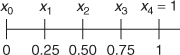
, ![]() . We divide the interval
. We divide the interval ![]() into n equal subintervals of width h, by the points
into n equal subintervals of width h, by the points ![]() where
where ![]()
Let ![]() be the corresponding values of y. In this method, the derivatives in the differential equations are replaced by their finite difference approximations, namely,
be the corresponding values of y. In this method, the derivatives in the differential equations are replaced by their finite difference approximations, namely,

Substituting these values in the given differential equation we get a difference equation, which can be solved using the boundary conditions.
Note: (1) is called forward difference approximation, where as (2) is a central difference approximation for yi′ and (3) is called central difference approximation for yi″.
WORKED EXAMPLES
Example 1
Using the finite difference method, find y(0.25), y(0.5) and y(0.75) satisfying the differential equation ![]() subject to the boundary conditions
subject to the boundary conditions ![]()
Solution
Given ![]()
Here ![]()
We know ![]()

 (1)
(1)
Given ![]()
If i = 1, then (1)
 (2)
(2)
If i = 2, then (1)
 (3)
(3)
If i = 3, then (1)
 (4)
(4)
Solve (2), (3), (4) to find y1, y2, y3
 (5)
(5)

![]()
Substituting in (3), ![]()
Thus, ![]()
Note: The equations (2), (3), (4) could be solved by Gauss elimination method.
Example 2
Solve the equation ![]() with the boundary conditions
with the boundary conditions ![]()
Solution
Given ![]()
![]()
∴
We shall divide the interval (0, 1) into 4 equal parts

We know ![]()
∴ the equation becomes


![]()

The equations are ![]() (1)
(1)
![]() (2)
(2)
![]() (3)
(3)
We use Gauss elimination method to find y1, y2 and y3
 (4)
(4)
 (6)
(6)

∴ ![]()
Example 3
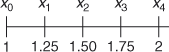
Solve xy′ + y = 0, y (1) = 1, y (2) = 2 with ![]() by using finite difference method.
by using finite difference method.
Solution
Given ![]()
∴ ![]() and
and ![]()
Since ![]()
![]()
We know

∴ the equation becomes
![]() , i = 1, 2, 3
, i = 1, 2, 3

![]()

![]()

![]()
∴ the equations are
![]() (1)
(1)
![]() (2)
(2)
![]() (3)
(3)
![]() (4)
(4)
![]() (5)
(5)
Adding, ![]()
![]() (6)
(6)
Subracting,
From(5), ![]()
From(6), ![]()
Thus
![]()
Exercises 10.1
- Solve the boundary value problem for
 by finite difference method
- Solve by finite difference method:
 by taking
- Using finite difference method, solve the differential equation

 with
with 
- Solve the equation
 , with
  taking
  using finite difference method.
 - Solve
 , given
  taking
  , using finite difference method.
 - Solve the equation
 and
and  using finite difference method.
Answers 10.1
(1)Take n = 4, y(0.5) = 0.1403 (2) 0.062, 0.250, 0.562 (3) –0.5556, –0.8889, –1
(5) 0.1389 (5) y(0,5) = 0.4706 (6) 0.2, 0.4, 0.6, 0.8
10.2 NUMERICAL SOLUTION OF PARTIAL DIFFERENTIAL EQUATIONS
We have seen numerical solution of second order ordinary differential equations by replacing the derivatives by the approximate differences. Similarly partial differential equations are also solved numerically by finite difference method. The partial derivatives appearing in the equation and the boundary conditions are replaced by their finite difference approximations. Thereby the given equation is converted into a system of a linear equations which are solved by iteration methods.
10.2.1 Classifications of Second Order Partial Differential Equations
Let u be a function of two independent variables x and y. Consider the partial differential equation of u of the form
 (1)
(1)
where A, B, C are functions of x and y or constants.
The second degree terms are linear whereas the part  may be non-linear. So the equation (1) is called a second order quasi-linear equation. Incase
  is linear then (1) is called a second order linear equation.
At a point (x, y) in the xy-plane, the equation (1) is
- elliptic if

- Parabolic if

- Hyperbolic if

Note:
- If at all points of a region R if
 , then the equation is elliptic or parabolic or hyperbolic in R.
 - It is quite possible an equation elliptic in one region may be parabolic in another region and hyperbolic in yet another region.
WORKED EXAMPLES
Example 1
Test the nature of (i) ![]()
(ii) ![]()
(iii) ![]()
(iv) ![]()
Solution
(i) Given ![]()
Here![]()

So, the equation is elliptic if ![]() ie. at all points on the right side of y-axis satisfying the equation. The equation is hyperbolic if
ie. at all points on the right side of y-axis satisfying the equation. The equation is hyperbolic if ![]() ie. at all points on the left side of y-axis satisfying the equation and parabolic if
ie. at all points on the left side of y-axis satisfying the equation and parabolic if ![]() ie at all points of y-axis satisfying the equation.
ie at all points of y-axis satisfying the equation.
(ii) Given ![]()
Here ![]()
![]()

So, the equation is hyperbolic in the ![]() and
and ![]() quadrants, elliptic in the
quadrants, elliptic in the ![]() and
and ![]() quadrants and parabolic at all points in the x-axis and y -axis which satisfy the equation.
quadrants and parabolic at all points in the x-axis and y -axis which satisfy the equation.
(iii) Given ![]()
Here ![]()

∴ the equation is hyperbolic for all (x, y) satisfying the equation
(iv) Given ![]()
Here ![]()
![]()
If ![]() then
then ![]() (as
(as ![]() for all
for all ![]() )
)
![]()
![]() or
or ![]() for all
for all ![]()
∴ the equation is hyperbolic if ![]() or
or ![]() and for all
and for all ![]()
If ![]() (as x2 > 0 ∴ x ≠ 0)
(as x2 > 0 ∴ x ≠ 0)
![]()
![]()
∴ the equation is elliptic if ![]() and
and![]()
If ![]() then
then ![]() or
or ![]()
∴ the equation is parabolic if ![]()
ie. on the y-axis or on the line ![]() or
or ![]()
Depending on the nature of the equations, methods of solving will differ.
Some well known equations, we consider for numerical solution are the following:
 is Laplace’s equation
ie. two dimensional heat equation in steady-state. It is elliptic type.
 Poisson’s equation.
It is elliptic type
 one dimensional wave equation.
It is hyperbolic type
 one dimensional heat equation.
It is parabolic type.
10.2.2 Finite Difference Approximations to Partial Derivatives
Consider a rectangular region in the xy-plane with sides parallel to the axes.
Divide this region into a network of rectangles of sides h and k units by drawing lines ![]()
![]() ,
, ![]() , 1, 2, 3, ... The points of intersection of these family of lines are called mesh points or lattice points or grid points.
, 1, 2, 3, ... The points of intersection of these family of lines are called mesh points or lattice points or grid points.
The point of intersection of ![]()
![]() is called the grid point
is called the grid point ![]()
If u is a function of two independent variables x and y then the value of ![]() at the grid point
at the grid point ![]() is denoted by
is denoted by ![]() . Thus
. Thus ![]()
Consider ![]() , where x is a variable and
, where x is a variable and ![]() is fixed then
is fixed then ![]() is single variable function.
is single variable function.
The Taylor’s series expansion of it in the neighbourhood of ![]() is
is
![]()
Put ![]() , then
, then
![]()
If h is small, we approximate as
![]() (1)
(1)
Replacing h by −h in (1), we get
(1) ∴ ![]() (2)
(2)
∴ 
This is called the forward difference approximation for ![]()
(2) ∴![]()
This is called the backward difference approximation for ![]()
(1) − (2) ∴![]()
∴![]()
This is called the central difference approximation to ![]() .
.
The central difference approximation is better than the forward and backward difference approximations.
In the same way the approximation for 2nd derivative is
![]()
Using backward difference approximations for ![]() and
and ![]() we get
we get
![]()
and ![]()
![]()

In the same way, the first and second partial derivatives w.r.to y can be obtained.
The forward difference approximation is
![]()
The backward difference approximation is
![]()
The central difference approximation is
![]()
and ![]()
Since ![]() , the above formulae can be written as
, the above formulae can be written as
![]() – forward difference
– forward difference
![]() – backward difference
– backward difference
![]() – central difference
– central difference
![]() – forward difference
– forward difference
![]() – backward difference
– backward difference
![]() – central difference
– central difference
![]()
![]()
10.2.3 Solution of Laplace Equation 
Given the equation ![]() , the solution
, the solution ![]() is satisfied by every point in a region subject to certain boundary conditions. Consider a rectangular region R for which
is satisfied by every point in a region subject to certain boundary conditions. Consider a rectangular region R for which ![]() is known at the boundary. For simplicity, take R to be a square region and divide it into small square regions of side h.
is known at the boundary. For simplicity, take R to be a square region and divide it into small square regions of side h.
Replacing ![]() and
and ![]() by differences
by differences


the equation becomes

![]() (1)
(1)
This shows that the value of u at any interior mesh point is the average value of the four adjacent mesh points on the lines through ![]()

ie. the average of the mesh point values above, below, left and right of ![]()
The formula (1) is called the standard five point formula (SFPF)
We know that Laplace equation remains invariant when the coordinate axes are rotated through ![]() . So we can also use the following formula.
. So we can also use the following formula.
![]() (2)
(2)
This shows that the value of ![]() is the average of the values of the four mesh points through the diagonals of
is the average of the values of the four mesh points through the diagonals of ![]() .
.

Figure 10.3
The formula (2) is called the diagonal five point formula (DFPF) as in Fig 10.3.
Now to find the initial values of u at the interior mesh points, we first find ![]() at the centre of the square by taking the mean of the 4 boundary values at the ends of the horizontal and vertical through
at the centre of the square by taking the mean of the 4 boundary values at the ends of the horizontal and vertical through ![]() .
.
![]()
![]()
Next we compute the initial values of the centers of the large squares with ![]() as a corner.
as a corner.
ie. we find ![]() by DFPF
by DFPF

The values at the remaining four mesh points ![]() are got by using SFPF
are got by using SFPF
Thus, we have

Having got all the values of ![]() , the accuracy of these values are improved by any one of the following iteration methods.
, the accuracy of these values are improved by any one of the following iteration methods.
1. Gauss Jacobi method:
If ![]() be the
be the ![]() iterative value of
iterative value of ![]() , then an iterative procedure to SFPF is given by
, then an iterative procedure to SFPF is given by
![]()
2. Gauss-Seidel method
The iterative formula for SFPF is given by
![]()
Here we use the latest available iterative values and hence the rate of convergence will be faster by this method. Infact, it is nearly twice faster than Jacobi method.
The application of Gauss-Seidel iteration to solve boundary value problems was due to Liebmann. So this method is known as Liebmann’s method.
Note: It can be proved that the error in the diagonal formula is four times than in the standard formula. So, as far as possible we use the standard five point formula.
WORKED EXAMPLES
Example 1
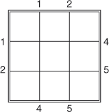
Determine by iteration method the values at the interior lattice points of a square region of the harmonic function u whose boundary values are given as shown in the figure below

Solution
Since u is harmonic, it satisfies Laplace equation
![]()
Let u1, u2, u3, … , u9 be the values of u at the interior points.
We find the initial values of u1, u2, …, u9.
Then by iteration improve these values.

We now start the iteration to improve these values. We start with u1 and proceed along horizontal.
Liebmann’s iteration formula is
![]()
I Iteration: SFPF


II Iteration:

III Iteration:


We notice that II and III iteration values are almost same
![]()
Remark: We have worked out elaborately. We can find the values of u’s at each grid point indicating the values at the point itself as in the table schematically.
Using the latest available values.

Example 2
Given the values of u(x, y) on the boundary of the square in the figure, evaluate the function u(x, y) satisfying the Laplace equation — 2u=0 at the pivotal points of the figure by Gauss-Seidel method.

Solution

To get the initial values of u1, u1, u3, u4 we can not use either SFPF or DFPF to find any values. So we shall assume u4 = 0 as the initial value.
Then

I Iteration:

II Iteration:

III Iteration:

IV Iteration:

V Iteration:
![]()
We take u1 = 1208, u2 = 792, u3 = 1042, u4 = 458
Example 3
By iteration method, solve the elliptic equation  over a square region of side 4, satisfying the boundary conditions


By dividing the square into 16 square mashes of side 1 and always correcting the computed values to two places of decimals, obtain the values of u at 9 interior pivotal points.
Solution
Given equation is ![]()
The boundary condition ![]() gives all boundary values zero on y-axis.
gives all boundary values zero on y-axis.
![]() ,
, ![]() means on x-axis the values are 0, 3, 6, 9, 12
means on x-axis the values are 0, 3, 6, 9, 12
![]() ,
, ![]() gives the values on x = 4 as 12, 13, 14, 15, 16.
gives the values on x = 4 as 12, 13, 14, 15, 16.
![]() ,
, ![]() means on y = 4 the boundary values are 0, 1, 4, 9, 16.
means on y = 4 the boundary values are 0, 1, 4, 9, 16.

Let us take the 9 interior grid points as u1, u2, u3, …, u9
First we have to find the initial values.

The other four values u2, u4, u6, u8 can be found by SFPF

I Iteration:

II Iteration:


III Iteration:


From the II and III iterations we can take the values of u correct to 2 places as
![]()
10.2.4 Poisson Equation
An equation of the form ![]() is called Poisson’s equation.(1)
is called Poisson’s equation.(1)
Proceeding as in Laplace equations we get the standard five point formula for poisson equation as
 (2)
(2)
By applying (2) at each interior mesh point, we obtain a system of linear equations in the Pivotal values i.j.
We solve by Gauss-Siedel method
method ![]()
WORKED EXAMPLES
Example 4
Solve the Poisson equation
∇2u = -10(x2 + y2 + 10), 0 ≤ x ≤ 3, 0 ≤ y ≤ 3, u = 0
on the boundary.
Solution
Given
Solve the Poisson equation
![]()
The region is a square bounded by x = 0, x = 3, y = 0, y = 3
Divide it into a square mesh with side h = 1.
Let u1, u2, u3, u4 be the values of u at the interior mesh points A, B, C, D
![]()
∴![]()

 (1)
(1)
 (2)
(2)
 (3)
(3)
 (4)
(4)
 (5)
(5)
![]() (2)′
(2)′
![]() (3)′
(3)′
![]() (4)′
(4)′
![]() (5)′
(5)′

Note: In the above problem ![]() which is symmetric in x and y. That is when x and y are interchanged the equation is not changed. So the function is symmetric about the line y = x. So the solution is symmetric about y = x.
which is symmetric in x and y. That is when x and y are interchanged the equation is not changed. So the function is symmetric about the line y = x. So the solution is symmetric about y = x.
The boundary conditions are also symmetric
∴ ![]()
This is the reason we got u1 = u4
This observation will be helpful in solving, when the number of mesh points are more in a square.
Example 5
Solve ![]() in the square mesh given u = 0 on the four boundaries dividing the square into 16 subsquares of length 1 unit.
in the square mesh given u = 0 on the four boundaries dividing the square into 16 subsquares of length 1 unit.
Solution
Given ![]()
Here h = 1
Let ![]() be the values of u at the interior grid points.
be the values of u at the interior grid points.
Choose u5 as origin and the x, y axes along the lines u5 u6 and u5 u2

Since the equation is symmetric in x and y and the boundary values are same when x and y are interchanged.
The values of u at the mesh points symmetric about y = x and about the axes will be the same

Hence we have to find only u1, u2, u5
The difference equation given by the SFPF for poisons equation is
 (1)
(1)
![]()
 (2)
(2)
 (3)
(3)
![]()
 (4)
(4)
![]()
![]()
Example 6
Solve the poisson equation ![]() Given that
Given that ![]()
Solution
Given ![]()
The equation is symmetric about x and y.
When x and y are interchanged it is unaffected and so symmetric about y = x.
The boundary conditions are also symmetric about y = x.
Let u1, u2, u3, u4 be the values of u at the mesh points.

∴ ![]()
The difference equation by SFPF is
 (1)
(1)

Now
 (1)
(1)
 (2)
(2)
 (3)
(3)
Substitute for u4 in (1) we get
 (4)
(4)
 (5)
(5)

10.3 ONE DIMENSIONAL HEAT EQUATION
The one dimensional heat equation is ![]()
(where c is the specific heat of the material, r is the density and k is the thermal conductivity).
It is a parabolic equation.
![]()
![]() (1)
(1)
We shall see two methods to solve for u(x, t) subject to the boundary conditions.
![]() (2)
(2)
![]() (3)
(3)
the initial conditions u(x, 0) = f(x), 0 < x < l(4)
10.3.1 Schmidt’s Method [Explicit Method]
Consider a rectangular mesh in the x-t plane with side lengths h in the x-direction and k in the t-direction. Let us denote the mesh point (x, y) = (ih, jk) as simply i, j.
Then we have the approximate relations of differences

Substituting in the equations (1), we get

∴ 
where![]() is the mesh ratio parameter.
is the mesh ratio parameter.
![]() (5)
(5)
The boundary conditions can be written as
![]()
and the initial condition can be written as
ux,0 = f(ih), i = 1,2,3,...
We choose the time interval k in such a way that the coefficient of ui,j in (5) is zero.
∴ 
Then the equation becomes
∴  (6)
(6)
This equation is called the Bender-Schmidt recurrence equation.
Note:
- The equation (6) gives the value of u at the (i, j + 1)th interior mesh point as the average of the values of u at the surrounding points xi + 1 and x i − 1 at previous time tj
- Schmidt method is called the explicit method because each subsequent computation u at t = tj + 1 is explicitly given from the previous u-value at t = tj
- Bender-Schmidt method is valid only for
 . To obtain more accurate results h should be small and hence k should be very small. This makes the computation pretty long because many time-intervals would be required to cover the prescribed region. The solution will become unstable if λ exceeds
  . The reason for this in the explicit method is the difference in orders of the finite-difference approximations for the spatial derivative
  and the time derivative
  .
.
The next method, proposed by Crank and Nicolson in 1947 is a technique that makes these finite difference approximations of the same order. This method does not restrict λ and also reduces the amount of computations.
10.3.2 Crank-Nicolson Method [Implicit Method]
One dimensional heat equations is ![]() (1)
(1)
where ![]() with boundary conditions
with boundary conditions ![]() and the initial condition
and the initial condition ![]()
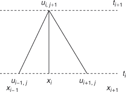
In this method ![]() is replaced by the average of its central-difference approximations on the jth and (j + 1)th time rows.
is replaced by the average of its central-difference approximations on the jth and (j + 1)th time rows.
∴ 
and ![]()
∴ the equation (1) becomes

Put ![]()
∴  (2)
(2)
This is called the Crank-Nicolson difference formula
Note:
- The left hand side of the formula contains three unknown values of u at the (j + 1)th time level while all the three values on the right hand side are known values of u at the jth level.
- Hence Crank-Nicolson formula is called a 2-level implicit relation because it does not give the value of u at t = tj + 1 directly in terms of u at t = tj
- To simplify the scheme, we choose k such that l = 1

- The Crank-Nicolson formula becomes
 (3)
(3)
If there are n internal mesh points on each row then the formula (2) gives a system of n simultaneous equations for the n unknown values in terms of the known boundary values. These equations can be soled by Gauss Seidel method. Similarly the values at the other internal mesh points on each row can be found.
WORKED EXAMPLES
Example 1
Solve ![]() and
and ![]() and, choosing h = k = 1 and using Bender-Schmidt formula find the values upto t = 5.
and, choosing h = k = 1 and using Bender-Schmidt formula find the values upto t = 5.
Solution

We have to choose ![]()
Bender-Schmidt recurrence formula for ![]() is
is

![]() (1)
(1)
x varies from 0 to 4 ∴ i = 0, 1, 2, 3, 4, j ≥ 0
The boundary value conditions become

We shall tabulate the meshpoint values of u
If j = 0, then ![]()
If i = 1, then ![]()
If i = 2, then ![]()
If i = 3, then ![]()
Similarly for j = 1, 2, 3, 4, 5. The values can be found and they are tabulated.
Now we shall tabulate the mesh point value of u

Example 2
Find the values of the function u(x, t) satisfying the differential equation ![]() and the boundary conditions
and the boundary conditions
u(0, t) = 0 = u(8, t) and ![]() at the points x = i, i = 0, 1, 2, 3, 4,...8 and
at the points x = i, i = 0, 1, 2, 3, 4,...8 and ![]() j = 0, 1, 2, 3, 4, 5.
j = 0, 1, 2, 3, 4, 5.
Solution
Given
![]()
![]()
Given i = 0, 1, 2, …, 8 and j = 0, 1, 2, 3, 4, 5
![]() , So,
, So, ![]()
Bender-Schmidt recurrence formula for ![]() is
is
![]()
The boundary conditions are ![]()
and 
For i = 0, 1, 2, …, 8, we get ![]()
![]()
These are the entries in the first row. Similarly we can find the other rows mesh points.
Now we shall tabulate the mesh point values of u

Example 3
Solve ![]() and u(x, 0) = 4(4 - x) choosing h = k = 1 using Bender-schmidt formula.
and u(x, 0) = 4(4 - x) choosing h = k = 1 using Bender-schmidt formula.
Solution
Given ![]()
Here a =1 ∴ a2 = 1 
The Bender-Schmidt formula for ![]() is
is
![]()
Since l = 1, the equation becomes
![]() (1)
(1)
Now x = ih = i, y = jk = j, ![]()
![]()

which are the first row mesh points. Similarly the other rows mesh points are computed.
Now we shall tabulate the mesh point values of u

Example 4
Solve ![]() with u(x, 0) = x (1 − x), 0 < x < 1,
with u(x, 0) = x (1 − x), 0 < x < 1,
u(0, t) = u(1, t) = 0 ![]() t > 0. Using explicit method with
t > 0. Using explicit method with ![]() for 3 time steps.
for 3 time steps.
Solution
Given ![]()
Here 
Here k is not given. We shall choose k such that ![]()
But 
![]()
Then Bender-Schmidt formula is
![]()
The boundary condition are ![]()
![]()
![]()
∴ 
These values are the first row mesh points.
For 3 time steps the mesh point values are given in the table

Example 5
Solve the equation ![]() with the conditions u(0, t) = 0, u(4, t) = 8 and
with the conditions u(0, t) = 0, u(4, t) = 8 and ![]() with the conditions u(0, t) = 0, u(4, t) = 8 and
with the conditions u(0, t) = 0, u(4, t) = 8 and ![]() , taking
, taking ![]() and
and ![]() upto 5 time units.
upto 5 time units.
Solution
Given ![]()

Since ![]() we have to use the general Schmidt’s formula
we have to use the general Schmidt’s formula
![]()
![]()
![]()
![]()

The boundary value conditions are u(0, t) = 0 ∴ u0,j = 0 ![]() j = 0, 1, 2, 3, 4, 5
j = 0, 1, 2, 3, 4, 5
When x = 4, t = 8, ![]()


Now we shall tabulate the mesh point value of u

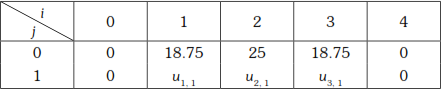
Example 6
Using Crank-Nicolson’s implicit scheme, solve 16 ut = uxx, 0 < x < 1, t > 0, given that u(x, 0) = 0, u(0, t) = 0, u(1, t) = 100t, compute u for one-time step.
Solution
Given uxx = 16 ut
Here 
Here (0, 1) is divided, choose ![]() .
.
Choose k such that 
Since l = 1, we use the simplified form of Crank-Nicolson formula

Boundary value conditions are

![]()
We have to compute the values of u for only one time step.
Put j = 0, i = 0, 1, 2, 3, 4.


Substituting for u1 and u3 in (2), we get
![]()


Example 7
Solve  given that u(x, 0) = 20, u(0, t) = 0, u(5, t) = 100. Compute u for one time step with h=1 by Crank-Nicolson method.
Solution
Given ![]()
Here ![]()
k is not given, so choose k such that l = 1 
Since l = 1, the simplified Crank-Nicolson formula is used to compute only one time step.
![]() (1)
(1)
where x = i h = i, t = k j = j

On the line x = 0, u = 0 for all t. That is for all j

Using formula (1)

Substituting (5) in (4),
 (6)
(6)
Substituting (2) in (3),
 (7)
(7)


∴ ![]()
Example 8
Solve ![]() subject to the conditions u(x, 0) = sin p x, 0 ≤ x ≤ 1 u(0, t) = u(1, t) = 0, using Crank-Nicolson method taking
subject to the conditions u(x, 0) = sin p x, 0 ≤ x ≤ 1 u(0, t) = u(1, t) = 0, using Crank-Nicolson method taking ![]()
Solution
Given uxx = ut

Crank-Nicolson formula is
![]()
Since ![]() , we get
, we get
![]()
Multiply by 4,
 (1)
(1)
The boundary conditions are ![]()


We shall find one time step values.
Putting j = 0, i = 1 in (1), we get
∴  (1)
(1)
Putting j = 0, i= 2, in (1) we get,
∴ 

∴
Substituting in (1), we get ![]()
Thus we have computed the value of u for one time step.
![]()
Example 9
Using Crank-Nicolson scheme Solve ![]() given u(x, 0) = u(0, t) = 0, u(1, t) = t, choosing h = 0.5,
given u(x, 0) = u(0, t) = 0, u(1, t) = t, choosing h = 0.5, ![]()
Solution
Given ![]()
Here

So we have to use Crank-Nicolson general formula
![]()
Putting ![]()
Multiply by 2, ![]() (1)
(1)
![]()
The boundary value conditions are
∴ 
We shall find one-step values.

Putting j = 0, i = 1 in (1), we get

Example 10
Solve by Crank-Nicolson’s method ![]() for 0 < x < 1, t > 0 given that u(0, t) = 0, u (1, t) = 0 and u(x, 0) = 100x(1 - x). Compute u for one time step with
for 0 < x < 1, t > 0 given that u(0, t) = 0, u (1, t) = 0 and u(x, 0) = 100x(1 - x). Compute u for one time step with ![]()
Solution
Given uxx= ut
Here 
![]()
So, we choose k such that 
Since l = 1, we use Crank-Nicolson simplified formula
 (1)
(1)
The boundary value conditions are

We have to compute on time step values of u

Putting i = 1, j = 0 in (1), we get
 (2)
(2)
Putting i = 2, j = 0 in (1), we get
 (3)
(3)
Putting i = 3, j = 0 in (1), we get
![]()
![]() (4)
(4)
From (2) and (4), we get u1,1 = u3,1
∴ (3) ∴ u2,1 ![]()
∴ 4u2,1 ![]()
∴ 4u2,1 ![]() [Using (2)]
[Using (2)]
![]()
∴ ![]()
∴ u2,1 = 14.29
∴ ![]()
and u3,1 = 9.82
Thus ![]()
Example 11
Obtain the Crank-Nicholson finite difference method by taking ![]() Hence, find u(x, t) in the rod for two time steps for the heat equation
Hence, find u(x, t) in the rod for two time steps for the heat equation ![]() given u(x, 0) = sin px, u(0, t) = 0, u(1, t) = 0. Take h = 0.2.
given u(x, 0) = sin px, u(0, t) = 0, u(1, t) = 0. Take h = 0.2.
Solution
Given ![]()
For derivation of Crank-Nicholson formula for one dimensional heat equation ![]() where
where ![]() refer page [In this question c is a]
refer page [In this question c is a]
Here ![]() and h = 0.2
and h = 0.2
Now l = 1 
Since l = 1, we use the simplified Crank-Nicolson formula
![]() (1)
(1)
where x = i h = 0.2 i, t = k j = 0.04 j and 0 ≤ x ≤ 1
When x = 0, i = 0 and when x = 1, ![]() ∴ i = 0, 1, 2, 3, 4, 5
∴ i = 0, 1, 2, 3, 4, 5
The boundary value conditions are ![]()
![]()
and u(x, 0) = sin px ∴ u(0.2i, 0) = sinp (0.2i) = sin![]()

On the line x = 0, u = 0![]() t ie. when i = 0, u = 0
t ie. when i = 0, u = 0 ![]() j
j
and on the line x = 1, u = 0![]() j ie. when i = 5, u = 0
j ie. when i = 5, u = 0 ![]() j
j
For two time steps we have to compute for j = 0, 1, 2
∴ ![]()
∴ 
We shall tabulate the values

We shall now compute the unknown u’s.
Putting j = 0 in (1) we get the second row values of u’s
![]()
![]()
![]()
![]() (2)
(2)
Put i = 2, then ![]()
![]()
![]() (3)
(3)
Put i = 3, then ![]()
![]()
![]() (4)
(4)
Put i = 4, then ![]()
![]()
![]() (5)
(5)
Substituting (5) in (4) we get
![]()
![]()
∴![]()
∴![]() (6)
(6)
Now substituting (2) in (3), we get

∴![]() (7)
(7)
(6) × 15 ∴ 225u3,1 106.5945
(7) × 4 ∴ 16u3,1 − 60u2,1 = −28.4264
Subtracting we get, 209u3,1 = 135.0209 ∴ u3,1 = 0.6460
Substituting in (6), we get
15(0.6460) − 4u2,1 = 7.1063
∴ 4u2,1 = 15(0.6460) − 7.1063 = 2.5837
∴ ![]()

To find the third row values of u, put j = 1 in (1)
∴![]()
Put i = 1, then ![]()
![]()
⇒ ![]() (8)
(8)
Put i = 2, then ![]()
![]()
![]() (9)
(9)
Put i = 3, then ![]()
![]()
![]() (10)
(10)
Put i = 4, then ![]()
![]()
![]() (11)
(11)
Substituting (11) in (10) we get,
![]()
![]()
∴ ![]() (12)
(12)
Substituting (8) in (9), we get,
![]()
![]()
∴ ![]()
∴ ![]() (13)
(13)
(12) × 15 ∴ 225u3,2 − 60u2,2 = 72.402
(13) × 4 ∴ 16u3,2 − 60u2,2 = −19.3068
Subtracting we get, 209 u3,2 = 91.7088 ∴ u3,2 = 0.4388
∴ 15u2,2 = 4(0.4388) + 4.8267 = 6.5819 ∴ u2,2 = 0.4388
∴ ![]()
and
![]()
Thus the two time step values are given in the table

10.4 ONE-DIMENSIONAL WAVE EQUATION
One dimensional wave equation (of vibrating string) is
![]() (1)
(1)
This is hyperbolic type.
We shall solve this for u(x, t) using finite difference method subject to the boundary conditions.
u(0, t) = 0, u(l, t) = 0(2)
and the initial conditions
u(x, 0) = f (x), ut(x, 0) = 0(3)
Assume equal interval h for x variable and equal interval k for t variable and x = ih, t = jk and u(x, t) = u(ih, jk) = ui,j
We know the partial derivatives in terms of differences
![]()

∴ the equation (1) becomes

∴ ![]()
Let ![]() then the equation becomes
then the equation becomes
∴ 
∴ ![]() (4)
(4)
This equation is an explicit formula for the solution of the wave equation because it gives the value of u at t = tj + 1, explicitly in terms of the values of u at t = tj and t = tj − 1
The simplest form of the equation (4) is obtained by putting
![]()
∴ the equation (4) becomes,
![]() (5)
(5)
The boundary conditions are
![]()
and ![]() if l = nh
if l = nh
The initial conditions are u(x, 0) = f(x) ∴ u(ih, 0) = f(ih)
∴ ui ,0 = f(ih), i = 0, 1, 2, 3 ,…
We shall use central difference approximation for
![]()
When t =0, ut(x,0) = 0 ∴ ![]() ⇒
⇒ ![]()
When j = 0, ![]()
∴ ![]() for all i
for all i
Putting j = 0 in (5), we get ![]()
![]()
∴−1,0
∴ ![]()
For i = 1, 2, 3, …, we get the values of u in the second row.
Note: The period of vibration of the string of length l given by ![]() is
is ![]() we have to find the values of u at the mesh points for one period, unless otherwise specified.
we have to find the values of u at the mesh points for one period, unless otherwise specified.
WORKED EXAMPLES
Example 1
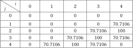
Solve 16uxx = utt, u(0, t) = u(5, t) = 0, u(x, 0) = x2(5 - x), ut(x, 0) = 0 taking h = 1 and upto one half of the period of vibration.
Solution
Given 16uxx − utt = 0
Here a2 = 16 ∴ a = 4.
Now ![]()
Choose l = 1 and h = 1, then ![]()
Since l = 1, the simplest difference equation is
![]() (1)
(1)
Now x = ih =i, t = jk = ![]() u(x, y) = u
u(x, y) = u ![]() = ui,j
= ui,j
From the boundary conditions u(0, t) = u(5, t) = 0, it is obvious 0 ≤ x ≤ 5 and length of the string l = 5
∴ period of vibration ![]()
Half the period = 1.25 secs.
So, we have to find values of t upto t = 1.25 ∴ ![]() = 1.25 ∴ j = 5
= 1.25 ∴ j = 5
![]() (2)
(2)
![]() (3)
(3)
![]()
∴ ![]() (4)
(4)
When t = 0, ![]() ∴
∴ ![]()
Since ![]() t = 0 ∴ j = 0
t = 0 ∴ j = 0
When j = 0, ![]() (5)
(5)
(2) ∴ ![]()
(3) ∴ ![]()
(4) ∴ ![]()
Putting j = 0 in (1), we get ![]()
![]() [Using (5)]
[Using (5)]
∴−1,0
∴ ![]() (6)
(6)

Put i = 1, ![]()

To fill up the 3rd row put j = 1 in (1)
∴ ![]()
Putting i = 1, 2, 3, 4, we get

To fill up the 4th row put j = 2 in (1)
∴ ![]()
Putting i = 1, 2, 3, 4 we get

To fill up the 5th row put j = 3 in (1)
![]()
Putting i = 1, 2, 3, 4, we get

To fill up the last row put j = 4 in (1)
![]()
Putting i = 1, 2, 3, 4, we get

Example 2
Solve the wave equation ![]()

and ![]() using h = k = 0.1 for 3 time steps.
using h = k = 0.1 for 3 time steps.
Solution
Given ![]()
Here a2 = 1 ∴ a = 1. h = k = 0.1
∴ ![]()
Since l = 1, the simplest equation is ![]() (1)
(1)
x = ih = (0.1)i, t = j k = (0.1)j, u(x, y) = ![]()
Since 0 ≤ x ≤ 1, x = 1 ∴ 0.1 i = 1 ∴ i = 10. So i = 0, 1, 2, ..., 10
Since t takes 3 steps, j = 0, 1, 2, 3
Given 
∴ ![]()


When t = 0, u(x, 0) = 0 ∴ ![]()
∴ ![]()
Now t = 0 ∴ j = 0
When j = 0, ![]()
(1) ∴
∴ 
∴ ![]()
Putting i =1, 2, ..., 9, we get


To find the values of u in the third row put j = 1 in (1)
![]()
Putting i = 1, 2, 3, …, 9, we get

To find the values of u in the 4th row put j = 2 in (1)
![]()
Putting i = 1, 2, ..., 9, we get

Example 3
Approximate the solution to the wave equation ![]() u(0, t) = 0, u(1, t) = 0, t > 0, u(x, 0) = sin2p x, 0 £ x £ 1 and
u(0, t) = 0, u(1, t) = 0, t > 0, u(x, 0) = sin2p x, 0 £ x £ 1 and ![]() 0 £ x £ 1 with Δx = 0.25 and Δt = 0.25 for 3 time steps.
0 £ x £ 1 with Δx = 0.25 and Δt = 0.25 for 3 time steps.
Solution
Given ![]()
Here a2 = 1 ∴ a =1; Δx = h = 0.25, Δt = k = 0.25
∴ ![]()
Since l = 1, the difference equation is
![]() (1)
(1)
![]()
![]()
Since ![]() i varies from 0 to 1 and
i varies from 0 to 1 and ![]()
We have to compute for 3 time steps. ∴ j = 0, 1, 2, 3
![]()
∴ ![]() (2)
(2)
u(0, t) = 0 for t > 0 ∴ u0,j = 0, j = 1, 2, 3 (3)

∴ ![]() (4)
(4)
∴ 
So we have the first row values of u.

To find second row mesh point values of u.
When t = 0 ut (x,0) = 0 ∴ ![]() ∴
∴ ![]()
When j = 0, j = 0]
When j = 0, (1) ∴ ![]()
![]()
∴ ![]()
∴ ![]() (5)
(5)
Putting i = 1, 2, 3, we get

To find the third row values of u, put j = 1 in (1)
∴ ![]()
Putting i = 1, 2, 3, we get

To find the fourth row values of u, put j = 2 in (1)
∴ ![]()
Putting i = 1, 2, 3, we get,

Example 4
Solve numerically 4uxx = utt with the boundary conditions u(0, t) = 0, u(4, t) = 0, t > 0 and the initial conditions ut(x, 0) = 0, u(x, 0) = x(4 − x), taking h = 1 for four time steps.
Solution
Given 4uxx = utt
Here a2 = 4 ∴ a = 2; h = 1
We shall choose k such that l = 1 ∴ ![]()
Since l = 1, the difference equation is
![]() (1)
(1)
![]()
From boundary condition, 0 ≤ x ≤ 4 and so i = 0, 1, 2, 3, 4
![]() (2)
(2)
Since we have to compute for 4 time steps j = 0, 1, 2, 3, 4
 (3)
(3)
∴ ![]() (4)
(4)
∴ ![]() [From (2)]
[From (2)]
and ![]() [From (3)]
[From (3)]
From (4), ![]()
So we have the first row values of u

Now to find other rows mesh point values of u
When t = 0, ![]() ∴ ui,j −1= 0
∴ ui,j −1= 0
When j = 0 j = 0]
∴ ![]() (5)
(5)
When j = 0, (1) ∴ ![]()
= ![]() [Using (5)]
[Using (5)]
∴ ![]()
∴ ![]()
When i = 1, ![]()
When i = 2, ![]()
When i = 3, ![]()
To find the values of u in the third row put j = 1 in (1)
∴ ![]()
Putting i = 1, 2, 3 we get

To find the values of u in the 4th row, put j = 2 in (1)
∴ ![]()
Putting i = 1, 2, 3, we get

To find the values of u in the 5th row, put j = 3 in (1)
∴ ![]()
Putting i = 1, 2, 3, we get

Exercises 10.2
(I) Elliptic equations:
- Solve uxx + uyy = 0 for the following mesh with boundary values as shown in the figure. Iterate until the maximum difference between the successive values at any point is less than 0.005.
- Solve uxx + uyy = 0 numerically for the following mesh with boundary conditions as shown below.

- Solve
 in the square mesh given u = 0 on the four boundaries dividing the square into 16 subsquares of length 1 unit.
- 0 over the square region of side n, satisfying the boundary condition
- 0, 0 ≤ y ≤ 4 (ii) u(4,y) = 12 y ≤ 4
- 3x, 0 ≤ y ≤ 4 (iv) u(x,4) = x2, 0 ≤ y ≤ 4.
- 8 + 2y, u(x, 0) =
 , u(x, 4) = x2 with

-
(II) Parabolic equations:
- (6) Solve
 subject to the conditions u(x, 0) =
 , u(0, t) = u(1, t) = 0
Using Schmidt method taking

- (7) Solve uxx = 32 ut = taking h = 0.25 for t > 0, 0 < x < 1 and u(x, 0) = 0, u(0, t) = 0, u(1, t) = t using Schmidt method.
- (8) Using Crank-Nicolson method solve uxx = 16 ut , 0 < x < 1, t > 0 given u(x, 0) = 0, u(0, t) = 0 and u(1, t) = 100 t, choosing
 .
. - − Nicoloson method
 0 < x < 2, t > 0, u (0, t) = u (2, t) = 0, t > 0 and u(x, 0)
  using h = 0.5, k = 0.25 for two time steps.
 - (10) Using Crank-Nicolson method solve ut = uxx in
 , t > 0, given u(0, t) = 0 u(l, t)
 - and u(x, 0) =

- Take h = 0.1 and find u for one step in t.
(III) Hyperbolic equations:
- 0.5, with spacing of 0.1 subject to y (0, t) = 0, y(1, t) = 0, yt (x, 0) = 10 − x).
- − x2),
 (x, 0) = 0, u(0, t) = u(1, t) = 0, t > 0 by finite difference method for one time step with h = 0.25.
 - (13) Solve
 0 < x < 1, t > 0, given u(x, 0) = 0, ut (x, 0) = u(0, t) = 0 and u(1, t) = 100 sin p t. Compute u for 4 time steps with h = 0.25.
 - − utt = 0 for u at the pivotal points, given u(0, t) = u(5, t) = 0, ut(x, 0) = 0 and
- u(x,0) =
 for one half period of vibration.
 - (15) Solve the boundary value problem utt = uxx = 0 with the conditions u(0, t) = u(1, t) = 0, u(x, 0)
 and ut(x, 0) = 0 taking h = k = 0.1 for
  . Compare your solution with the exact solution at x = 0.5 and t = 0.3.
 - Answers 10.2
- 1.999, 2.999, 3.999 (2) u1 = u4 = 1.333, u2 = u3= 1.6667
- − 3 (4) 2.37, 5.59, 9.87, 2.88, 6.13,
- − 2, u5 = − 2 9.88, 3.01, 6.16, 9.51
- 4.9, u3 = 9, u4 = 2.07, u5 = 4.69,
- u6 = 8.07, u7 = 1.57, u8 = 3.71, u9 = 6.57]
- (6)

- (7)

- 1.7857, u 2 = 7.1429, u3 = 26.7857
- u1 = 0.2857, u2 = 0.1429, u3 = 0.2857, u4 = 0.0816, u5 = 0.1837, u6 = 0.0816
- (10)

- (11)

- (12)

- (13)
- (14)

- Find the exact solution when t = 0.3 or j = 3

- (6) Solve
Short Answer Questions
- 0.
- 2. Identify the type of the equation fxx + 2fxy + fyy = 0.
- 3. Classify the partial differential equation uxx + 2uxy + 4uyy = 0, x > 0, y > 0.
- 4. For what values of x and y, the equation xfxx + yfyy = 0, x > 0, y > 0 is elliptic?
- 5. Obtain the finite difference approximation for the differential equation

- 6. Name at least two numerical methods that are used to solve one dimensional diffusion equation.
- 7. Write down Laplace equation and its finite difference analogue and the standard five point formula.
- 8. State the explicit finite difference scheme for one dimensional wave equation

- 9. Find the explicit finite differences scheme for one dimensional wave equation

- 10. Write down the Crank-Nicolson formula to solve ut = uxx.
- 11. Write down the implicit formula to solve one dimensional heat flow equation

- 12. Why is Crank - Nicolson’s scheme is called an implicit scheme?
- 13. What type of equations can be solved by using Crank-Nicolson’s formula?
- 0.
- 15. State Leibmann’s iteration process formula.
- 16. Write down the finite difference form of the Poisson equation ∴2u = f(x, y).
- 17. Write down the Schemidt’s explicit formula for solving heat flow equation.
- − aut = 0.
- 19. Write down the Crank-Nicolson difference scheme to solve uxx = aut with u(0, t) = T0, (l, t) = T1 and the initial condition as u(x, 0) = f(x).
- Write down the Forward difference approximation to ux(x0, y0).
- 21. Write down the backward difference approximation of ux(x0, y0).
- 22. Write down the finite difference approximation to uxx, where u = u(x, y) taking, h, k as the step sizes at the point (x, y).
C H A P T E R
10

