Chapter 11. Advanced Data Management

What You’ll Learn in This Chapter

• How write data into buffers and textures directly from your shaders.

• How to get OpenGL to interpret data in a flexible manner.

• How to directly share data between the CPU and the GPU.

So far in this book you have learned how to use buffers and textures to store data that your program can use. Buffers and textures can be bound to the OpenGL pipeline for writing in the form of transform feedback or framebuffers. In this chapter, we’ll cover a few of the more advanced techniques involving data and data management. We’ll dive into texture views, which allow you to apply more than one interpretation to data. We’ll take a deeper look at texture compression and use a compute shader to compress texture data on the GPU. We’ll also look at ways to share data directly between the CPU and the GPU, including how to arbitrate which processor owns the data at any particular time.

• The number of textures that a single shader can access is limited to the number of texture units that the OpenGL driver supports. The minimum requirement in OpenGL 4.5 is 16 units per stage. Although some implementations support 32 units per stage or more, this is still a fairly small amount.

• Your application needs to spend time binding and unbinding textures between draws. This makes it difficult to combine draws that otherwise would be able to use the same state.

To get around these problems, we can use a feature known as bindless textures. This functionality will be available to your application if OpenGL reports that the GL_ARB_bindless_texture extension is supported. This extension allows you to get a handle for a texture and then use that handle directly in your shaders to refer to the underlying texture without having to bind it to a texture unit. Additionally, it allows you to control the list of textures that will be available to your shaders. In fact, it requires this because, as you are no longer using texture binding points, OpenGL has no way of knowing which textures might be used and therefore need to be in memory before running your shaders.

Once you have created a texture, you can get a handle for it by calling either of the following functions:

Click here to view code image

GLuint64 glGetTextureHandleARB(GLuint texture);
GLuint64 glGetTextureSamplerHandleARB(GLuint texture, GLuint sampler);

The first function produces a handle representing the texture named in the texture parameter, using its built-in sampler parameters. The second function returns a handle representing texture and the sampler given in sampler as if that pair had been bound to a texture unit. Notice that both glGetTextureHandleARB() and glGetTextureSamplerHandleARB() return a GLuint64 64-bit integer value. You will need to pass those values into your shaders to use them. The simplest way to do so is to put the value into a uniform block. That is, you declare one of GLSL’s sampler types in a uniform block declaration and then place the 64-bit handle into a buffer and use it to back the uniform block. Listing 11.1 shows an example of making this type of declaration.

Click here to view code image

#version 450 core

#extension GL_ARB_bindless_texture : require

layout (binding = 0) uniform MYBLOCK
{
    sampler2D theSampler;
};

in vec2 uv;
out vec4 color;

void main(void)
{
    color = texture(theSampler, uv);
}

Listing 11.1: Declaring samplers inside uniform blocks

As you can see from Listing 11.1, once you have enabled the bindless texture exension and then declared samplers in your uniform blocks, using the samplers is identical to the ordinary non-bindless usage.

Before running any shaders that access bindless textures, you need to tell OpenGL which textures might be used. There is no specific upper limit to the number of textures that might be in use—you are limited only by the capabilities of the underlying OpenGL implementation and the resources available to it. When you bind textures to traditional texture units, OpenGL can determine from what’s bound what might be used. However, once you eliminate binding points, you become responsible for making this notification yourself. To put a texture onto the “might be used” list, call

Click here to view code image

void glMakeTextureHandleResidentARB(GLuint64 handle);

To take a texture off the resident list, call

Click here to view code image

void glMakeTextureHandleNonResidentARB(GLuint64 handle);

In both cases, the handle parameter is the handle returned from a call to either glGetTextureHandleARB() or glGetTextureSamplerHandleARB(). The term resident refers to the underlying memory used to store the texture’s data. You can think of the list of resident textures as a set of virtualized binding points that are not accessible to you, but which OpenGL uses to track what needs to be in memory at any given point in time.

With the simple example shown in Listing 11.1, which moves a single sampler declaration into a uniform block, this might not seem like a particularly useful feature, especially considering the additional steps required—create the texture, get its handle, make it resident, and so on. However, consider what happens if we put multiple textures inside a single uniform block, or even embed them inside a structure. Then textures become data just like regular constants. Now your material definitions can simply include textures, for example.

The bindlesstex example demonstrates the use of bindless textures. We adapted a shader to modulate the lighting of each pixel by a texture, the handle to which is stored in a uniform. Listing 11.2 shows the fragment shader from the example.

Click here to view code image

#version 450 core

// Enable bindless textures
#extension GL_ARB_bindless_texture : require

// Output
layout (location = 0) out vec4 color;

// Input from vertex shader
in VS_OUT
{
    vec3 N;
    vec3 L;
    vec3 V;
    vec2 tc;
    flat uint instance_index;
} fs_in;

// Material properties - these could also go in a uniform buffer
const vec3 ambient = vec3(0.1, 0.1, 0.1);
const vec3 diffuse_albedo = vec3(0.9, 0.9, 0.9);
const vec3 specular_albedo = vec3(0.7);
const float specular_power = 300.0;

// Texture block
layout (binding = 1, std140) uniform TEXTURE_BLOCK
{
    sampler2D      tex[384];
};

void main(void)
{
    // Normalize the incoming N, L, and V vectors
    vec3 N = normalize(fs_in.N);
    vec3 L = normalize(fs_in.L);
    vec3 V = normalize(fs_in.V);
    vec3 H = normalize(L + V);

    // Compute the diffuse and specular components for each fragment
    vec3 diffuse = max(dot(N, L), 0.0) * diffuse_albedo;
    // This is where we reference the bindless texture
    diffuse *= texture(tex[fs_in.instance_index], fs_in.tc * 2.0).rgb;
    vec3 specular = pow(max(dot(N, H), 0.0), specular_power) * specular_albedo;

    // Write final color to the framebuffer
    color = vec4(ambient + diffuse + specular, 1.0);
}

Listing 11.2: Declaring samplers inside uniform blocks

As you can see in Listing 11.2, we declared a uniform block with 384 textures in it. This is significantly more than the number of traditional texture binding points supported by the OpenGL implementation upon which the sample was developed, and more than an order of magnitude greater than the number of samplers supported in a single shader stage.

To actually generate 384 textures, we use a simple procedural algorithm during application start-up to produce a pattern and then modify it slightly for each texture. For each of the 384 textures, we create the texture, upload a different set of data into it, get its handle, and make it resident with a call to glMakeTextureHandleResidentARB(). We place the handles into a buffer object that will be used as a uniform buffer by the fragment shader. The code is shown in Listing 11.3.

Click here to view code image

glGenBuffers(1, &buffers.textureHandleBuffer);
glBindBuffer(GL_UNIFORM_BUFFER, buffers.textureHandleBuffer);

glBufferStorage(GL_UNIFORM_BUFFER,
                NUM_TEXTURES * sizeof(GLuint64) * 2,
                nullptr,
                GL_MAP_WRITE_BIT);

GLuint64* pHandles =
    (GLuint64*)glMapBufferRange(GL_UNIFORM_BUFFER,
                                0,
                                NUM_TEXTURES * sizeof(GLuint64) * 2,
                                GL_MAP_WRITE_BIT | GL_MAP_INVALIDATE_BUFFER_BIT);

for (i = 0; i < NUM_TEXTURES; i++)
{
    unsigned int r = (random_uint() & 0xFCFF3F) << (random_uint() % 12);
    glGenTextures(1, &textures[i].name);
    glBindTexture(GL_TEXTURE_2D, textures[i].name);
    glTexStorage2D(GL_TEXTURE_2D,
                   TEXTURE_LEVELS,
                   GL_RGBA8,
                   TEXTURE_SIZE, TEXTURE_SIZE);
    for (j = 0; j < 32 * 32; j++)
    {
        mutated_data[j] = (((unsigned int *)tex_data)[j] & r) | 0x20202020;
    }
    glTexSubImage2D(GL_TEXTURE_2D,
                    0,
                    0, 0,
                    TEXTURE_SIZE, TEXTURE_SIZE,
                    GL_RGBA, GL_UNSIGNED_BYTE,
                    mutated_data);
    glGenerateMipmap(GL_TEXTURE_2D);
    textures[i].handle = glGetTextureHandleARB(textures[i].name);
    glMakeTextureHandleResidentARB(textures[i].handle);
    pHandles[i * 2] = textures[i].handle;
}

glUnmapBuffer(GL_UNIFORM_BUFFER);

Listing 11.3: Making textures resident

To render all these textures on real objects, we created a simple test wrapper that uses another uniform block to store an array of transformation matrices; in the vertex shader, we then index into that array using gl_InstanceID. We also pass the instance index to the fragment shader of Listing 11.2, where it is used to index into the array of texture handles. This allows us to render a single object with an instanced drawing command. Each instance uses a different transformation matrix and a different texture. The resulting output is shown in Figure 11.1. This image is also shown in Color Plate 7.

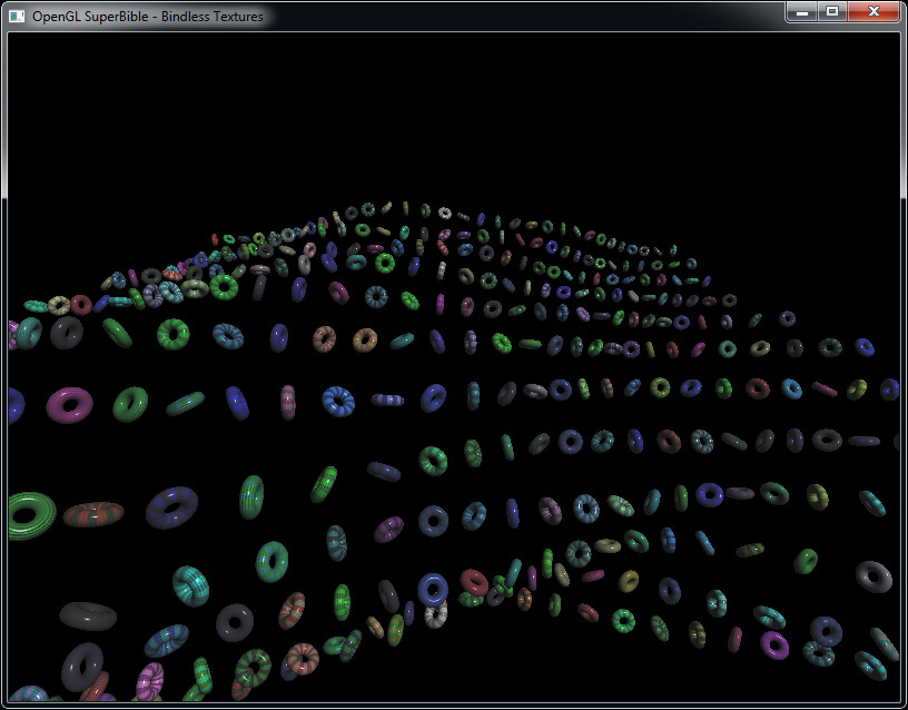
As you can see, each of the objects in Figure 11.1 has a different colored pattern on it. This pattern is created from the 384 unique textures. In an advanced application, each of these textures would originate from user-generated content and be unique rather than generated programmatically. Here, we have demonstrated that a single draw command can access hundreds of unique textures.

_RGBA8 format consumes 16 megabytes of memory just for the base mipmap level. A third of this amount of memory is consumed by the mipmap chain, making the requirements reach over 21 megabytes. A typical graphically intensive application might have tens or hundreds of these chains in use at a time, pushing the total memory requirements for the application into the hundreds of megabytes and possibly well into the multiple gigabytes range. However, even in such an application, it is unlikely that all of that data will be needed at the same time. Rather, objects that would normally have a high-resolution texture applied to them might be seen only from a distance, meaning that only the lower-resolution mipmaps might be used. Another common use case is atlas textures—textures that are used to apply details to irregular objects where not all of the rectangular texture space is used for image data.

To accomodate these kinds of scenarios, you can use the GL_ARB_sparse_texture extension. This extension allows textures to be sparsely populated, separating the logical dimensions of the texture from the physical memory space required to store its texels. In a sparse texture, the texture itself is divided into a number of square or rectangular regions known as pages. Each page can either be committed or uncommitted. When a page is committed, you can use it like an ordinary texture. When a page is uncommitted, OpenGL will not use any memory to store data for it. Reading from it under this circumstance will not return useful data, and any data you write to such a region will just be discarded.

Before you can use sparse textures, you need to make sure that OpenGL supports the GL_ARB_sparse_texture extension. Once you have determined that the extension is supported, you can create sparse textures using the glTextureStorage2D() function. To create a sparse texture, you need to tell OpenGL about your intention before allocating storage for the texture, by calling glTextureParameteri() with the GL_TEXTURE_SPARSE_ARB parameter. This is demonstrated in Listing 11.4.

Click here to view code image

GLuint tex;

// Create a new texture
glCreateTexture(1, &tex);

// Tell OpenGL that we want this texture to be sparse
glTextureParameteri(tex, GL_TEXTURE_SPARSE_ARB, GL_TRUE);

// Now allocate storage for the texture
glTextureStorage2D(tex, 14, GL_RGBA8, 16384, 16384);

Listing 11.4: Creating a sparse texture

The code in Listing 11.4 creates a 16,384 × 16,384 texel texture with a complete mipmap chain with an internal format of GL_RGBA8. Normally, this texture would consume a gigabyte of memory. This is the largest size of 2D texture that must be supported by OpenGL—larger textures may be supported but this is not guaranteed. Because the texture is sparse, however, the storage space is not consumed immediately. Only virtual space is reserved for the texture and no physical memory is allocated. To commit pages (that is, to allocate physical storage for them), we can call glTexPageCommitmentARB(), whose prototype is

Click here to view code image

void glTexPageCommitmentARB(GLenum target,
                            GLint level,
                            GLint xoffset,
                            GLint yoffset,
                            GLint zoffset,
                            GLsizei width,
                            GLsizei height,
                            GLsizei depth,
                            GLboolean commit);

glTexturePageCommitmentEXT() can commit and decommit pages into the sparse texture whose name is given in texture. The level parameter specifies in which mipmap level the pages reside. The xoffset, yoffset, and zoffset parameters give the offset, in texels, where the region to be committed or decommitted begins, and the width, height, and depth parameters specify the size of the region, again in texels. If the commit parameter is GL_TRUE, the pages are committed; if it is GL_FALSE, they are decommitted (freed).

All of the parameters—x offset, y offset, z offset, width, height, and depth—must be integer multiples of the page size for the texture. The page size is determined by OpenGL based on the internal format of the texture. You can determine the page size by calling glGetInternalformativ() and passing the tokens GL_VIRTUAL_PAGE_SIZE_X_ARB, GL_VIRTUAL_PAGE_SIZE_Y_ARB, and GL_VIRTUAL_PAGE_SIZE_Z_ARB to find the page size for the format in the x, y, and z dimensions, respectively. There may actually be more than one possible page size. glGetInternalformativ() can also be used to find out how many virtual page sizes are supported for a given format by passing the GL_NUM_VIRTUAL_PAGE_SIZES_ARB token. Listing 11.5 shows an example of determining the number of virtual page sizes and identifying what they are using glGetInternalformativ().

Click here to view code image

GLuint num_page_Sizes;
GLuint page_sizes_x[10];
GLuint page_sizes_y[10];
GLuint page_sizes_z[10];

// Figure out how many page sizes are available for a 2D texture
// with internal format GL_RGBA8
glGetInternalformativ(GL_TEXTURE_2D,
                      GL_RGBA8,
                      GL_NUM_VIRTUAL_PAGE_SIZES_ARB,
                      sizeof(GLuint),
                      &num_page_sizes);

// We support up to 10 internal format sizes -- this is hard-coded
// in the arrays above. We could do this dynamically, but it's unlikely
// that an implementation supports more than this number, so it's not really
// worth it.
num_page_sizes = min(num_page_sizes, 10);

// One call for each dimension
glGetInternalformativ(GL_TEXTURE_2D,
                      GL_RGBA8,
                      GL_VIRTUAL_PAGE_SIZE_X_ARB,
                      num_page_sizes * sizeof(GLuint),
                      page_sizes_x);
glGetInternalformativ(GL_TEXTURE_2D,
                      GL_RGBA8,
                      GL_VIRTUAL_PAGE_SIZE_Y_ARB,
                      num_page_sizes * sizeof(GLuint),
                      page_sizes_y);
glGetInternalformativ(GL_TEXTURE_2D,
                      GL_RGBA8,
                      GL_VIRTUAL_PAGE_SIZE_Z_ARB,
                      num_page_sizes * sizeof(GLuint),
                      page_sizes_z);

Listing 11.5: Determining supported sparse texture page sizes

If the number of page sizes returned when retrieving GL_NUM_VIRTUAL_PAGE_SIZES_ARB is zero, your OpenGL implementation doesn’t support sparse textures for the specified format and dimensionality of texture. If the number of page sizes is more than one, OpenGL will likely return the page sizes sorted into an order of its preference—probably based on memory allocation efficiency or performance under use. In that case, you’re probably best off to pick the first one. Some combinations don’t make a whole lot of sense. It is quite probable, for example, that all OpenGL implementations will return 1 for the page size in the z dimension when a format is used with a 2D texture, but they might return something else for a 3D texture. That is why the texture type is specified in the call to glGetInternalformativ().

Not only do the regions of the texture need to be committed and decommitted in page-size blocks (which is why the parameters to glTexturePageCommitmentEXT() need to be multiples of the page size), but the texture itself also needs to be an integer multiple of the page size. This holds only for the base level of the mipmap. As each mipmap level is half the size of the previous level, eventually the size of a mipmap level becomes less than a single page. This so-called mipmap tail is the part of the texture where commitment cannot be managed at the page level. In fact, the whole tail is considered to be either committed or uncommitted as a single unit. Once you commit part of a mipmap tail, the whole tail becomes committed. Likewise, once any part of the mipmap tail is decommitted, the whole thing becomes decommitted. As a side effect of this constraint, you cannot make a sparse texture whose base mipmap level is smaller than a single page.

When pages of a texture are first committed with a call to glTexPageCommitmentARB(), their contents are initially undefined. However, once you have committed them, you can treat them like part of any ordinary texture. You can put data into them using glTextureStorageSubImage2D(), or attach them to a framebuffer object and render into them, for example.

The sparsetexture application shows a simple example of using sparse textures. In this example, we assume that the page size for the texture is a factor of 128 texels for GL_RGBA8 data (which works out to 64K). First, we allocate a large texture consisting of 16 pages × 16 pages (which works out to 2048 × 2048 texels for a 128 × 128 page size). Then, on each frame, we use the frame counter to generate an index by switching a few of its bits around and then making pages resident or nonresident at the computed location. For pages made newly resident, we upload new data from a small texture that we load on start-up.

For rendering, we draw a simple quad over the entire viewport. At each point, we sample from the texture. When pages are resident, we get the data stored in the texture. Where pages are not resident, we receive undefined data. In this application, that’s not terribly important and we display whatever is read (even if it might be garbage). On the machine used to develop the sample application, the OpenGL implementation returns zero for unmapped regions of data. The implementation of the rendering loop is shown in Listing 11.6.

Click here to view code image

static int t = 0;
int r = (t & 0x100);
int tile = bit_reversal_table[(t & 0xFF)];

int x = (tile >> 0) & 0xF;
int y = (tile >> 4) & 0xF;

// If page is not resident...
if (r == 0)
{
    // Make it resident and upload data
    glTexPageCommitmentARB(GL_TEXTURE_2D,
                           0,
                           x * PAGE_SIZE, y * PAGE_SIZE, 0,
                           PAGE_SIZE, PAGE_SIZE, 1,
                           GL_TRUE);
    glTexSubImage2D(GL_TEXTURE_2D,
                    0,
                    x * PAGE_SIZE, y * PAGE_SIZE,
                    PAGE_SIZE, PAGE_SIZE,
                    GL_RGBA, GL_UNSIGNED_BYTE,
                    texture_data);
}
else
{
    // Otherwise make it nonresident
    glTexPageCommitmentARB(GL_TEXTURE_2D,
                           0,
                           x * PAGE_SIZE, y * PAGE_SIZE, 0,
                           PAGE_SIZE, PAGE_SIZE, 1,
                           GL_FALSE);
}

t += 17;

Listing 11.6: Simple texture commitment management

The output of the sparsetexture sample is shown in Figure 11.2. As you can see in the figure, there are missing data blocks in the texture and only parts of the texture are visible in the screenshot.

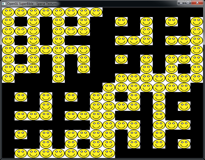
The example given in sparsetexture is very simple and serves only to demonstrate the feature. In a more advanced application, we may use multiple sparse textures and combine their results, or use secondary textures to store meta-data about the residency of our main texture. For example, a common use case for sparse textures is streaming texture data over time.

Consider the scenario where you have a large level of a game that consumes hundreds of megabytes of texture data. When players first start the game, they are placed at a specific part of the map—most of the map will not be visible to them and many of the parts of the map will be far from them and therefore rendered at a low resolution. Making the players wait for all textures to be loaded (which could be a considerable amount of time if the textures are on a remote server across the Internet, or stored on slower media such as DVDs) would make for a poor user experience. However, delaying loading a texture until the first time the user sees an object can cause stuttering and in-game slowdowns, which also negatively affect the user’s experience.

Using sparse textures can resolve the issue nicely. The idea is to allocate every texture as sparse and then populate only the lowest-resolution mipmap levels of all of them before the game starts. As the lowest mipmap levels consume exponentially less storage space than the texture base levels, the time taken to load them is substantially less than if all textures needed to be loaded ahead of time. When the user first sees part of the map, we can then guarantee that at least a low-resolution version of the texture is available in the smallest mipmap level. In many cases, this works very well because objects start far from the user and need only their lowest mipmap levels anyway. As the user gets closer and closer to an object, the higher-resolution mipmap levels for that object’s textures can be loaded.

To properly sample from a texture, we need to clamp the level of detail that OpenGL will use to guarantee that we’re going to pull from only committed texels. To do that, we need to know which pages are committed. This requires a second, level-of-detail texture, which we can sample from to find the lowest committed level-of-detail for a given texture coordinate. Listing 11.7 shows a snippet of shader code that samples from a sparse texture by calculating the required level-of-detail, fetching from the committed level-of-detail texture, and then clamping the result to the highest available level (the lowest-resolution level) before sampling from the actual sparse texture.

Click here to view code image

uniform sampler2D uCommittedLodTexture;
uniform sampler2D uSparseColorTexture;

vec4 sampleFromSparse(vec2 uv)
{
    // First, get the available levels of detail for each of the
    // four texels that make up our filtered sparse texel.
    vec4 availLod = textureGather(uCommitedLodTexture, uv);

    // Calculate the level-of-detail that OpenGL would like
    // to sample from.
    vec2 desiredLod = textureQueryLod(uSparseColorTexture, uv);

    // Find the maximum of the available and desired LoD.
    float maxAvailLod = max(max(availLod.x,
                                availLod.y),
                            max(availLod.z,
                                availLod.w));

    // Compute the actual LoD to be used for sampling.
    // Note that this is the maximum value of LoD, representing the
    // lowest-resolution mipmap -- our application fills the texture
    // from lowest to highest resolution (highest to lowest LoD).
    float finalLod = max(desiredLod.x, max(desiredLod.y, maxAvailLod));

    // Finally, sample from the sparse texture using the computed LoD.
    return textureLod(uSparseColorTexture, uv, lod);
}

Listing 11.7: Sampling a sparse texture with clamped level-of-detail (LoD)

By reusing some of the code in Listing 11.7, you can get the GPU to provide feedback to the application about which texture pages are needed. Bind an image as writable and, when the desired level-of-detail (the desiredLod variable in Listing 11.7) is lower (that is, higher resolution) than the available level-of-detail, write the desired level-of-detail into the image. Periodically, read the content of this image back into your application¹ and scan it. You can use this information to decide what to stream in next.

1. To avoid GPU stalls, remember to leave a good amount of time between updating the image containing the desired level-of-detail and reading it back.

The RGTC texture compression format is one of the simpler formats supported by OpenGL. It has been part of the core specification for a number of years and is designed to store one- and two-channel images. Like other similar formats, it is block based, and each compressed block of data represents a 4 × 4 texel region of the image. For simplicity, we will assume that source images are a multiple of 4 texels wide and high. Only two-dimensional images are supported by the RGTC format, although it should be possible to stack a number of 2D images into an array texture or even a 3D texture. It is not possible to render into a compressed texture by attaching it to a framebuffer object.

The RGTC specification includes signed and unsigned, one- and two-component formats:

• GL_COMPRESSED_RED_RGTC1 represents unsigned single-channel data.

• GL_COMPRESSED_SIGNED_RED_RGTC1 represeents signed single-channel data.

• GL_COMPRESSED_RG_RGTC2 represents unsigned two-channel data.

• GL_COMPRESSED_SIGNED_RG_RGTC2 represents signed two-channel data.

We will begin by discussing the GL_COMPRESSED_RED_RGTC1 format. This format represents each 4 × 4 block of texels using 64 bits of information. If each input texel is an 8-bit unsigned byte, then the input data comprises 128 bits, producing a compression ratio of 2:1. The principle of this compression format (like many others) is to take advantage of the limited range of values that are likely to appear inside a small region of image data. If we find the minimum and maximum values appearing inside a block, then we know that all texels within that block fall within that range. Therefore, all we need to do is determine how far along that range a given texel is, and then encode that information for each texel rather than the value of the texel itself. For images with smooth gradients, this works well. Even for images with hard edges, each texel might be at opposite ends of the range and still produce a reasonable approximation to the edge.

Figure 11.3 demonstrates this principle graphically. After finding the minimum and maximum values of the pixels in a small block, we encode them as the endpoints of a line. This is represented by the y axis in Figure 11.3. The line extends from the y coordinate of the highest value on the graph to the y coordinate of the graph. Then, we quantize the x axis into a number of small regions and encode the region into which each texel falls in our compressed image. Each of these regions is represented by a different hatching pattern on the graph. Each of the texel values (represented by the vertical bars) then falls into one of the four regions defined by subdividing the line. It is the index of this region that is encoded for each texel, along with the values of the endpoints of the line that are shared by the whole block.

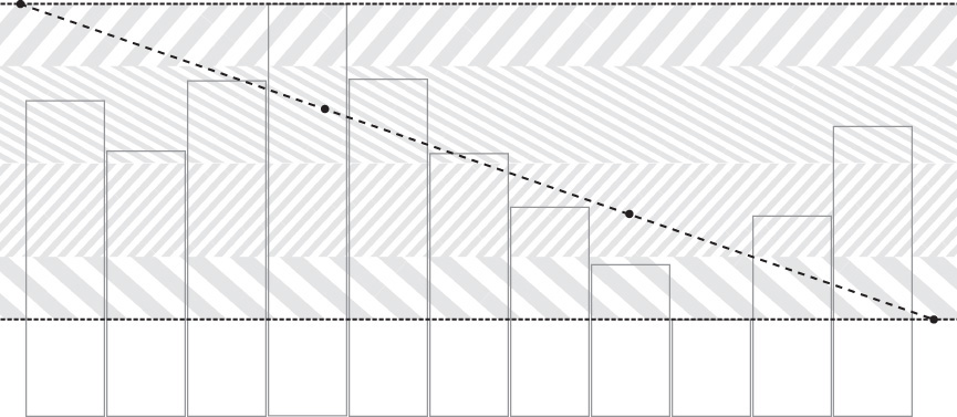
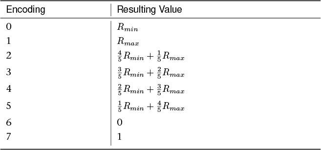
Each 64-bit (8-byte) block begins with two bytes representing the values of the two endpoints of the line. This leaves 48 bits (64 − 16) in which to encode the values of the pixels. As there are 16 pixels in a 4 × 4 block, that leaves 3 bits for each texel. In the straightforward encoding, this divides our range into 8 pieces. Note that in the case where the minimum and maximum values of the texels in a block are within 8 gray levels of each other, this encoding scheme will produce lossless compression. The encoding is not quite direct, however. Table 11.1 shows how the value of each 3-bit field (values of 0 through 7) corresponds to the encoded texel value.

There is a special case that takes advantage of the fact that we can store additional information in the first 2 bytes of the block beyond only the endpoints of our line. If we store the mimimum value first, followed by the maximum value, then the usage for the 3 bits for each texel described previously holds. However, if we store the maximum value first, and then the minimum value, we can reverse the order of the regions, continuing to encode the same data, except we can now use this ordering to signal a slightly different encoding.

As you can see from Table 11.2, there are fewer regions that can be represented using this second encoding, but the values 0 and 1 can be exactly represented regardless of the values of the endpoints.² This allows us to use this encoding to better represent a solid black line against a lighter, textured background, for example.

2. Remember, this is a normalized texture, so 1 here represents a value of 255 when interpreted as an integer.

In effect, the first two values in the block can be used to define an eight-entry palette. Upon reading the block, we compare the two endpoint values and generate the appropriate palette. Then, for each 3-bit field in the remaining 6 bytes of compressed data, we generate a single output texel by using it as an index into the palette we just generated.

To take advantage of the dual encodings supported by RGTC, we’re going to write two variants of our compressor—one that produces data in the first encoding and one that produces data in the second encoding—and then decide, for each block, which of the two encodings to use based on the computed per-pixel error. We will look at the first encoding initially, and then see how we can modify it to produce the second encoding. The design is intended to produce an encoder that can execute in a compute shader. While we could try to compress a single block using many theads in parallel, the goal is not necessarily to encode a single block as quickly as possible, but rather to compress a large image quickly. As each block can be compressed independently of all others, it makes sense to write a compressor that runs inside a single thread, and then compress as many blocks as possible in parallel. This simplifies the encoder because compressing each block essentially becomes a single-threaded operation with no need to share data or synchronize with other work items.

First, our compressor loads a 4 × 4 block of texels into a local array. Because we are operating on single-channel data, we can use GLSL’s textureGatherOffset function to read 4 texels from a 2 × 2 block in one function call. The texture coordinate passed to textureGatherOffset must lie in the center of the 2 × 2 region. Listing 11.8 shows the code that gathers 16 texels’ worth of data in four calls to textureGatherOffset.

Click here to view code image

void fetchTexels(uvec2 blockCoord, out float texels[16])
{
    vec2 texSize = textureSize(input_image, 0);
    vec2 tl = (vec2(blockCoord * 4) + vec2(1.0)) / texSize;

    vec4 tx0 = textureGatherOffset(input_image, tl, ivec2(0, 0));
    vec4 tx1 = textureGatherOffset(input_image, tl, ivec2(2, 0));
    vec4 tx2 = textureGatherOffset(input_image, tl, ivec2(0, 2));
    vec4 tx3 = textureGatherOffset(input_image, tl, ivec2(2, 2));

    texels[0] = tx0.w;
    texels[1] = tx0.z;
    texels[2] = tx1.w;
    texels[3] = tx1.z;

    texels[4] = tx0.x;
    texels[5] = tx0.y;
    texels[6] = tx1.x;
    texels[7] = tx1.y;

    texels[8] = tx2.w;
    texels[9] = tx2.z;
    texels[10] = tx3.w;
    texels[11] = tx3.z;

    texels[12] = tx2.x;
    texels[13] = tx2.y;
    texels[14] = tx3.x;
    texels[15] = tx3.y;
}

Listing 11.8: Fetching a block of texels using textureGatherOffset

Once we have read the 16 texels of information from the source image, we can construct our palette. To do so, we will find the minimum and maximum values of the texels in the block, and then compute the resulting output color value for each of the eight possible encodings of data. Note that it’s not necessary to sort the values of the texels—all we need to know is what the minimum and maximum values present are, not the order in which they occur. Listing 11.9 shows how we produce the palette for the first encoding. We will cover the second encoding shortly.

Click here to view code image

void buildPalette(float texels[16], out float palette[8])
{
    float minValue = 1.0;
    float maxValue = 0.0;
    int i;

    for (i = 0; i < 16; i++)
    {
        maxValue = max(texels[i], maxValue);
        minValue = min(texels[i], minValue);
    }

    palette[0] = minValue;
    palette[1] = maxValue;
    palette[2] = mix(minValue, maxValue, 1.0 / 7.0);
    palette[3] = mix(minValue, maxValue, 2.0 / 7.0);
    palette[4] = mix(minValue, maxValue, 3.0 / 7.0);
    palette[5] = mix(minValue, maxValue, 4.0 / 7.0);
    palette[6] = mix(minValue, maxValue, 5.0 / 7.0);
    palette[7] = mix(minValue, maxValue, 6.0 / 7.0);
}

Listing 11.9: Generating a palette for RGTC encoding

Once we have our palette, we need to map each of the texels in the block to one of the palette entries. To do this, we simply run through each palette entry and find the one with the closest absolute value to the texel under consideration. Listing 11.10 shows how this is done.

Click here to view code image

float palettizeTexels(float texels[16], float palette[8], out uint entries[16])
{
    uint i, j;
    float totalError = 0.0;

    for (i = 0; i < 16; i++)
    {
        uint bestEntryIndex = 0;
        float texel = texels[i];
        float bestError = abs(texel - palette[0]);
        for (j = 1; j < 8; j++)
        {
            float absError = abs(texel - palette[j]);
            if (absError < bestError)
            {
                bestError = absError;
                bestEntryIndex = j;
            }
        }
        entries[i] = bestEntryIndex;
        totalError += bestError;
    }

    return totalError;
}

Listing 11.10: Palettizing an RGTC block

Once we have palettized our block, we need to pack the resulting colors and indices into our output data structure. Remember, each compressed block starts with the two endpoint colors followed by 3 bits for each texel in the block. Three is not a convenient number when we’re running on machines that operate natively on powers of 2. Also, GLSL has no 64-bit type, which means we’ll need to use a uvec2 to hold our data. Worse yet, one of our 3-bit fields will need to straddle the boundary between the components of our uvec2. However, the resulting function still isn’t overly complex and is shown in Listing 11.11.

Click here to view code image

void packRGTC(float palette0,
              float palette1,
              uint entries[16],
              out uvec2 block)
{
    uint t0 = 0x00000000;
    uint t1 = 0x00000000;

    t0 = (entries[0] << 0u) +
         (entries[1] << 3u) +
         (entries[2] << 6u) +
         (entries[3] << 9u) +
         (entries[4] << 12) +
         (entries[5] << 15) +
         (entries[6] << 18) +
         (entries[7] << 21);

    t1 = (entries[8] << 0u) +
         (entries[9] << 3u) +
         (entries[10] << 6u) +
         (entries[11] << 9u) +
         (entries[12] << 12u) +
         (entries[13] << 15u) +
         (entries[14] << 18u) +
         (entries[15] << 21u);

     block.x = (uint(palette0 * 255.0) << 0u) +
               (uint(palette1 * 255.0) << 8u) +
               (t0 << 16u);
     block.y = (t0 >> 16u) + (t1 << 8u);
}

Listing 11.11: Packing an RGTC block

Earlier, we mentioned that a second encoding for RGTC textures allows exact representation of 0 and 1 without making them one of the endpoints of the palette. Essentially, the only modification to our compressor is to produce a second palette, but rather than using the true maximum and minimum values from the block, we use the minimum and maxium values from the block that are not either 0 or 1. A modified version of our buildPalette function is shown in Listing 11.12.

Click here to view code image

void buildPalette2(float texels[16], out float palette[8])
{
    float minValue = 1.0;
    float maxValue = 0.0;
    int i;

    for (i = 0; i < 16; i++)
    {
        if (texels[i] != 1.0)
        {
            maxValue = max(texels[i], maxValue);
        }
        if (texels[i] != 0.0)
        {
            minValue = min(texels[i], minValue);
        }
    }

    palette[0] = maxValue;
    palette[1] = minValue;
    palette[2] = mix(maxValue, minValue, 1.0 / 5.0);
    palette[3] = mix(maxValue, minValue, 2.0 / 5.0);
    palette[4] = mix(maxValue, minValue, 3.0 / 5.0);
    palette[5] = mix(maxValue, minValue, 4.0 / 5.0);
    palette[6] = 0.0;
    palette[7] = 1.0;
}

Listing 11.12: Generating a palette for RGTC encoding

Did you notice how our palettizeTexels function returns a floating-point value? That value is the accumulated error across all texels in the block when converted from their true values to the values available from our palette. Once we have generated the second palette using the buildPalette2 function from Listing 11.12, we palettize the block once with the first palette (using the first encoding scheme) and once with the second palette (using the second encoding scheme). Each function returns the error—we use the resulting palettized block from whichever function returns the smaller error metric.

After the packRGTC function shown in Listing 11.11 has run, the resulting uvec2 holds the 64-bit compressed block distributed across its two components. All we need to do now is write the data out to a buffer. Unfortunately, there is no way to write the image data directly into a compressed texture that can be immediately used by OpenGL. Instead, we write the data into a buffer object. That buffer can then be mapped so that the data can be stored to disk, or it can be used as the source of data in a call to glTexSubImage2D().

To store our image data, we’ll use an imageBuffer uniform in our compute shader. The main entry point of our shader looks like Listing 11.13.

Click here to view code image

void main(void)
{
    float texels[16];
    float palette[8];
    uint entries[16];
    float palette2[8];
    uint entries2[16];
    uvec2 compressed_block;

    fetchTexels(gl_GlobalInvocationID.xy, texels);

    buildPalette(texels, palette);
    buildPalette2(texels, palette2);

    float error1 = palettizeTexels(texels, palette, entries);
    float error2 = palettizeTexels(texels, palette2, entries2);

    if (error1 < error2)
    {
        packRGTC(palette[0],
                 palette[1],
                 entries,
                 compressed_block);
    }
    else
    {
        packRGTC(palette2[0],
                 palette2[1],
                 entries2,
                 compressed_block);
    }

    imageStore(output_buffer,
               gl_GlobalInvocationID.y * uImageWidth + gl_GlobalInvocationID.x,
               compressed_block.xyxy);
}

Listing 11.13: Main function for RGTC compression

As noted, the RGTC compression scheme is ideally suited to images that have smooth regions. Figure 11.4 shows the result of applying this type of compression to the distance field texture from Subsection 13, along with magnified portions of the image. On the left is the original, uncompressed image. On the right is the compressed image. As you can tell, there is little or no visible difference between the two. In fact, the demo in Subsection 13 uses a texture compressed using RGTC.

However, OpenGL supports a few more data types that are not represented directly in C. They include the special data type GL_HALF_FLOAT and a number of packed data types. The first of these, GL_HALF_FLOAT, is a 16-bit representation of a floating-point number.

The 16-bit floating-point representation was introduced in the IEEE 754-2008 specification and has been widely supported in GPUs for a number of years. Modern CPUs do not generally support it, but this is slowly changing with specialized instructions appearing in newer models. The 32-bit floating-point format consists of a single sign bit, which is set when the number is negative; 8 exponent bits, which represent the remainder of the number to be raised to the exponent; and that remainder, which is known as the mantissa and is 23 bits long. In addition, there are several special encodings to represent things like infinity and undefined values (such as the result of division by zero). The 16-bit encoding is a simple extension of this scheme, in which the number of bits assigned to each component of the number is reduced. There is still a single sign bit, but there are only 5 exponent bits and 10 mantissa bits. Just as 32-bit floating-point numbers have a higher dynamic range than 32-bit integers, so 16-bit floating-point numbers have a higher dynamic range than 16-bit integers.

Regardless of the packing of bits within a 16-bit floating-point number, the raw bits of the number can still be manipulated, copied, and stored using other 16-bit types such as unsigned short. So, for example, if you have three channels of 16-bit floating-point data, you can extract any of the channels’ data using a simple pointer dereference. The 16-bit type is still a natural length for computers that work with nice, round powers of 2. For the packed data formats, however, this is not true. Here, OpenGL stores multiple channels of data packed together into single, natural data types. For example, the GL_UNSIGNED_SHORT_5_6_5 type stores three channels—two 5-bit channels and one 6-bit channel—packed togther into a single unsigned short quantity. The C language has no representation for this arrangement. To get at the individual components, you need to use bitfield operations, shifts, masks, or other techniques directly in your code (or helper functions to do it for you).

The OpenGL names for packed formats are broken into two parts. The first part consists of one of our familiar unsigned integer types—GL_UNSIGNED_BYTE, GL_UNSIGNED_SHORT, or GL_UNSIGNED_INT. It tells us the parent unit in which we should manipulate data. The second part of the name indicates how the data fields are laid out inside that unit. This is the _5_6_5 part of GL_UNSIGNED_SHORT_5_6_5. The bits are laid out in most significant to least significant order, regardless of the endianness of the host machine, and appear in the order of the components as seen by OpenGL. So, for GL_UNSIGNED_SHORT_5_6_5, the 5 most significant bits are the first element of the vector, the next 6 bits are the second element, and the last 5 bits are the third element of the vector. Sometimes, however, the order of the vector elements can be reversed. In this case, _REV is appended to the type name. For example, the type GL_UNSIGNED_SHORT_5_6_5_REV uses the 5 most significant bits to represent the third channel of the vector, the next 6 bits to represent the second channel, and the final 5 least significant bits to represent the first channel of the result vector.

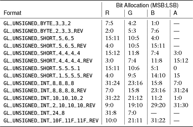
Table 11.3 shows the complete list of packed data formats supported by OpenGL. In addition to the formats listed in Table 11.3, the GL_FLOAT_32_UNSIGNED_INT_24_8_REV format interleaves a floating-point value in a first 32-bit word with an 8-bit quantitiy stored in the 8 least significant bits of a second 32-bit word. This format and GL_UNSIGNED_INT_24_8 are commonly used to store interleaved depth and stencil information. Further, the shared exponent format GL_UNSIGNED_INT_5_9_9_9_REV could be considered a packed data format, but is also a form of compression and is covered in “Shared Exponents.”

In Figure 11.5 you can almost see the centers of the texels. In fact, the texel centers keep their original values from the underlying texture and the reproduced texel value given to your shader linearly moves from one texel to another. The jarring artifacts, appearing almost as lines running through the centers of the texels, is due to the discontinuity in the gradient of the intensity of the image. Between each texel center, the image intensity is interpolated in a straight line. As the texture coordinate passes through the center of a texel, that straight line suddenly changes direction. This change in direction is the artifact that you can see in the image. For clarification, take a look at Figure 11.6, which represents a one-dimensional texture in graph form.

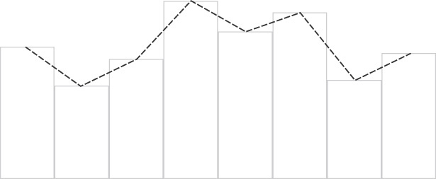
The graph in Figure 11.6 illustrates the problem well. Imagine that this graph represents a one-dimensional texture. Each bar of the graph is a single texel, and the dotted line is the result of interpolating between them. We can clearly see the interpolated lines between the texel centers and the abrupt change in direction that each new segment of the graph creates. Instead of using this linear interpolation scheme, it would be much better if we could move smoothly from one texel center to another, leveling off as we reach the texel center and avoiding the discontinuity at each.

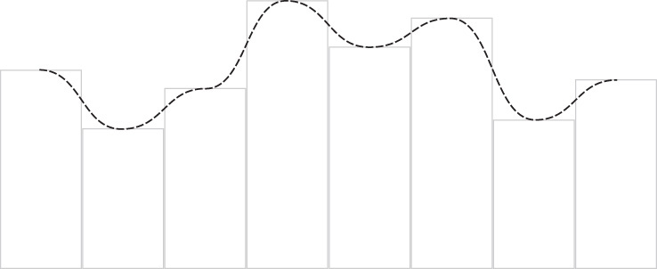
As luck would have it, we do have a smooth interpolation function—smoothstep does exactly what we want. If we take the graph of Figure 11.6 and replace each of the linear sections with a smoothstep curve, we get a much nicer fit to the texel centers and, more importantly, no gradient discontinuities. We can see this result in Figure 11.7.

The question, then, is how to use this type of interpolation in our shaders. If you look closely at your linear interpolation function, OpenGL first takes your texture coordinate, which represents the extent of the texture in the range 0.0 to 1.0, and scales it to the size of the texture. The integer part of the resulting number is used to select a texel from the texture, and the fractional part of the number is used as a weight to linearly interpolate it with its neighbors. Given a fractional part f, the weights used to blend two adjacent texels are (1 − f) and f (which sum to 1). What we’d like to do is replace f with another number—the result of the smoothstep function. Of course, we still need the weights for adjacent texels to sum to 1, and we’d like the number to start from 0 and reach 1 at the same time as f would have. Finally, we’d like the rate of change (the gradient) of this function to be 0 at its ends, which is also a property of the smoothstep function.

We can do all of this in our shader. All we need is a little arithmetic and a single, linear texture lookup (the same as we had before). We’re going to modify the texture coordinates used for sampling from the texture to cause the graphics hardware to use our weights for interpolation rather than its own.

Listing 11.14 shows the GLSL code to do this math for us. As you can see, only a few lines of code are needed and the number of texture lookups is the same as it was before. In many OpenGL implementations, there should be almost no performance penalty for using this function instead of regular texture filtering.

Click here to view code image

vec4 hqfilter(sampler2D samp, vec2 tc)
{
    // Get the size of the texture we'll be sampling from
    vec2 texSize = textureSize(tex, 0);

    // Scale our input texture coordinates up, move to center of texel
    vec2 uvScaled = tc * texSize + 0.5;

    // Find integer and fractional parts of texture coordinate
    vec2 uvInt = floor(uvScaled);
    vec2 uvFrac = fract(uvScaled);

    // Replace fractional part of texture coordinate
    uvFrac = smoothstep(0.0, 1.0, uvFrac);

    // Reassemble texture coordinate, remove bias, and
    // scale back to 0.0 to 1.0 range
    vec2 uv = (uvInt + uvFrac - 0.5) / texSize;

    // Regular texture lookup
    return texture(samp, uv);
}

Listing 11.14: High-quality texture filtering function

The result of sampling a texture using the function given in Listing 11.14 is given in Figure 11.8. As you can see, filtering the texture with this function produces a much smoother image. Texels are slightly more visible, but they have smooth edges and there are no obvious discontinuities at texel centers.