6
INTEGER PROGRAMMING: BINARY-CHOICE MODELS
An integer programming model is a linear program with the requirement that some or all of the decision variables must be integers. In principle, we could distinguish between linear programs with integer variables and nonlinear programs with integer variables, but the latter are extremely difficult to optimize and generally beyond the capability of Solver. Therefore, we focus on the role of integer variables in what would otherwise be linear programming models. Thus far, we have paid limited attention to whether the decision variables take on integer values. In Chapter 3, we pointed out that in special network models, integer solutions are guaranteed. In other cases, we encountered integer solutions without explicitly requiring integers, so there seemed to be no need to discuss integrality. In still other cases, we seemed to be content with fractional solutions, especially when the decision variables were scaled. In this chapter, the role of integer values takes center stage.
This chapter first describes how Solver handles integer programs. Next, we explore the basic capital budgeting model as a way of introducing binary variables and developing some intuition for the effects of integer requirements on decision variables. Then, in the remainder of the chapter, we look at models characterized by binary choice. In these optimization models, all decisions are of a yes/no variety. Other uses of binary variables are covered in the next chapter.
Before we discuss how to handle the integer requirement using Solver, we return briefly to the subject of integers in linear programs. Recall that one of the three conditions of linearity is divisibility—that is, the fact that fractional values make sense for decision variables. Consider Example 2.1, the allocation model for chairs, desks, and tables. As it turned out, the optimal solution contained no chairs, 160 desks, and 120 tables, so that the decision variables happened to all be integers. Suppose instead that the problem had been posed with only 1800 assembly hours available, rather than the 2000 of the base case. Then the optimal product mix would have been 13.33 chairs, 220 desks, and no tables. Is the fractional number of chairs meaningful?
At first glance, it may seem to make no sense to talk about one-third of a chair in the product mix. Certainly, if we were interested in the tactical implications of the solution, it would not make sense for us to produce one-third of a chair to help meet demand (or to count on the profit that the fractional chair would generate). However, there are two interpretations of the fraction that do make sense. For one, we should be willing to round off. That is, we might interpret the optimal solution as 13 chairs and 220 desks. This solution would use less capacity than the optimal solution but would clearly be feasible. Another possibility might be to round up the number of chairs to 14, leaving desks at 220. Although this rounded-up solution violates the precise statement of capacity, the violation is on the order of one-tenth of a percent in the case of assembly capacity and half a percent in the case of machining capacity. Because we are unlikely to “know” the given information in this problem to a precision of one part in a thousand, we may well accept the rounded-up product mix as an implementable solution.
A second interpretation is also possible. We might want to think of the model as representing a routine weekly planning model that specifies conditions in a typical or average week. In that context, when we encounter a figure like 13.33 in the optimal mix, we could interpret it as a long-run average. That is, the fractional value prescribes a 3-week cycle with 13 chairs in weeks 1 and 2 and 14 chairs in week 3. Thus, rounded-off values and planning averages provide us with two interpretations that might allow us to tolerate fractional answers to linear programs when fractions seem impractical in literal terms. In addition, we might be primarily interested in understanding the economic priorities in the optimal solution (as discussed in Chapter 4), and the details of the decision variables might be of secondary importance. Keeping in mind that linear programming models are usually guides to decisions, rather than fully automated substitutes for decisions, we might well be satisfied with noninteger solutions to most of our linear programs. Nevertheless, some cases arise in which only integers will suffice. In those cases, the requirement of integer values is crucial, and it influences how we use Solver.
Broadly speaking, three types of integer programming models are of interest. The first type is essentially a linear program but with a requirement that some or all of the variables must be integers. For example, a decision variable might correspond to the number of times in a production schedule that a piece of equipment is shut down for a maintenance check. In this instance, a value such as 2.59 will not suffice; we must have an integer. For this purpose, we designate some variable in the model as an integer variable.
The second type is a model in which some of the key decisions are of the yes/no variety. For example, a decision variable might correspond to whether or not we purchase a parcel of land. In this instance, we model our decision with a variable that is allowed to be only zero or one. We refer to such a decision as a binary choice, because there are only two alternatives, and we use binary variables to represent the decision. Binary variables are integer variables that are limited to the values 0 or 1. In this chapter, we mainly focus on models involving binary choice.
The third type is a model that contains certain relationships that we might not normally think of as linear. For example, suppose that we are contemplating a plant expansion in which we may add a new manufacturing line to the factory. If we proceed with the expansion, then we can produce a particular component internally. If we don’t expand, then we will have to buy the component from an external vendor. In other words, our make/buy alternatives are contingent on the decision to expand. Such a contingency is an example of a logical or qualitative constraint, but we can capture it in a model if we use binary variables to represent the decision to expand and the decision to produce components in house. Other kinds of qualitative constraints can often be represented using binary variables, and in the next chapter, we focus on models involving logical constraints.
6.1 USING SOLVER WITH INTEGER REQUIREMENTS
To illustrate how to use Solver for integer programming, let’s consider the staffing problem faced by a call center. Daily requirements for staff are usually developed from studies of congestion in the service system. Then an optimization model helps determine how large a staff is needed to cover the staffing requirements.
At the call center, seven different work shifts are possible under union rules. Each shift starts a 5-day work period on a particular day. For example, suppose we use SU to represent the number of employees who start work on Sunday, MO for the number who start work on Monday, and so on. These variables can make sense only if their values are integers. The constraints require that the number of employees assigned to work a given day must be at least as large as the daily minimum. For example, the number working on Thursday (SU + MO + TU + WE + TH) must be greater than or equal to 15, and a similar constraint applies for each of the other days of the week. In addition, the total salary cost for a week plays the role of the objective function. The algebraic model, shown below, is a variation on the staff-scheduling model introduced in Chapter 2:

Figure 6.1 shows the complete spreadsheet model. It is also a variation of the spreadsheet model for staff scheduling introduced in Chapter 2. When we treat this model as a linear programming problem, the model specification is as follows:


Figure 6.1 Spreadsheet model for Example 6.1.
As shown in Figure 6.1, Solver produces a solution containing some fractions (e.g., 3.667 employees starting on Monday) and a total cost of $8656.67.
The application of Solver to integer programming models, once they are formulated, is relatively straightforward. Solver treats the requirement that a variable must be an integer as an additional constraint. Along with the familiar constraint types ≤, ≥, and =, the drop-down menu in the Add Constraint window also permits int and bin. The int constraint designates a variable to be integer valued, while the bin constraint designates a variable to be either 0 or 1 (binary valued). To produce an integer solution in Example 6.1, we add a constraint that designates the decision variables to be integers, as shown in Figure 6.2. The specification of the model in the Solver Parameters window is shown in Figure 6.3, where we can see the explicit designation of integer variables.

Figure 6.2 Declaring integer variables in Example 6.1.

Figure 6.3 Model specification for Example 6.1.
Once we build the model and designate particular variables as integer or binary, the next step is to examine the options available in the Solver Parameters window. By clicking on the Options button, we reach the Options window, shown in Figure 6.4. Here, we set the Integer Optimality option to zero; the other entries can be left at their default values. At some other setting for Integer Optimality, such as 5%, Solver is guaranteed to find a solution that is no worse than 5% away from the optimum, as measured by the objective function. Clearly, we would prefer to find the very best solution, and this calls for an Integer Optimality parameter of zero. However, in some large models, a small Integer Optimality level may require the solution procedure to take a great deal of time. Therefore, we sometimes keep the level at 5% while debugging a large model, and we leave it at that level if we find that solution times are prohibitively long otherwise. If Solver can locate a solution at the 5% level in a reasonable amount of time, we can experiment further by lowering the parameter toward zero.

Figure 6.4 Options window in Solver.
With the integer variables designated and the Integer Optimality parameter set, Solver produces an optimal solution, shown in Figure 6.5, with a total cost of $8790. On the surface, at least, there is no intuitive reason why we would have anticipated this result based on the solution to the linear program. It is not, for example, a rounded-off version of the optimal solution. Thus, by using the integer programming capability in Solver, Callum Communications can meet its staffing requirements with minimum salary cost.

Figure 6.5 Optimal integer solution to Example 6.1.
As suggested by this example, integer programming models look just like linear programming models, except for the fact that certain variables are constrained to be integer valued. The differences occur within Solver, not in the spreadsheet model. Moreover, finding a solution with Solver simply requires the user to take two additional steps beyond the typical procedure for solving linear programs—that is, designating integer variables and setting the Integer Optimality parameter. If the only role of integers in a model is to avoid fractional values in what otherwise would be a normal linear program, then the formulation principles we covered in Chapters 2 and 3, along with the int constraint, are likely to suffice. That was the case in Example 6.1.
In some applications, such as the call center model, all of the variables are constrained to be integers. This type of model is sometimes called a pure integer program. In other cases, certain variables may be integers, but others are allowed to be fractional. A model containing both kinds of variables is called a mixed-integer program. Using Solver, the only difference between these two cases is the set of variables designated by the int constraint.
At the level of building models for use with Solver, integer programming may seem to be a minor technical extension of what we can already do with linear programming. However, as we explore the formulation of integer programs using binary variables in this chapter and the next, a very different picture emerges. The opportunity to use binary variables provides access to a class of models that is actually very different from linear programming.
The solution algorithm within Solver for handling integer programs is generically known as a branch-and-bound procedure. At the end of this chapter, we take a look at how such a procedure works.
6.2 THE CAPITAL BUDGETING PROBLEM
A binary variable, which takes on the values 0 or 1, can represent a yes/no decision—that is, a decision that represents a choice between taking an action and not taking it. We sometimes think in terms of discrete projects, where the decision to undertake the project is represented by the value 1 and the decision to forego the project is represented by the value 0. A classic example arises in conjunction with the capital budgeting problem, as illustrated by the Newton Corporation.
The problem facing the Newton Corporation can be posed as an allocation model with one constraint, as shown below, with objective function and constraint scaled to represent millions of dollars:

A spreadsheet model for this problem is shown in Figure 6.6. (A feasible, but suboptimal set of choices is displayed.) If we treat the model as if it were a simple linear program, we can specify the problem as follows:


Figure 6.6 Linear program for Example 6.2.
In the discussion that follows, we elaborate on the development and interpretation of this integer programming model as it is derived from the linear programming model. Our purpose is to develop some intuition for binary variables in optimization models, and we won’t elaborate in the same way for the other modes we introduce later.
The optimal NPV in the linear program for Example 6.2 appears to be $8 million, as shown in Figure 6.7, but the solution would require the selection of project P4 five times. However, none of the projects can be implemented more than once. In particular, it is not possible to buy the same parcel of land and build new headquarters five times; obviously, that activity can be done only once.

Figure 6.7 Optimal solution to the linear program for Example 6.2.
To prevent any project from being implemented several times, we can require each of the variables to be no greater than 1. If we optimize the model as a linear program, imposing an upper bound of 1 on each of the variables, the maximum NPV comes to just under $7 million, as shown in Figure 6.8, but the optimal mix of projects is P1, P4, P5, and one-fifth of P3. However, none of the projects can be done in a fractional amount. In the case of P3, we cannot pay for a fraction of a stadium name; the project is indivisible and must be either accepted or rejected in its entirety. No partway adoption of any of the projects is possible. Therefore, we must use binary variables, as all-or-nothing variables, to represent choices.

Figure 6.8 Optimal solution to the linear program for Example 6.2 with ceilings of 1.
Having seen why a purely linear programming approach is unsuitable for the situation at the Newton Corporation, we add the constraint that each variable is binary. The model specification is as follows:

The optimal solution achieves a NPV of $6.6 million, achieved by accepting projects P1, P3, and P4, as shown in Figure 6.9. This figure represents the largest value that can be achieved with the five candidate projects from the allocation of a $40 million budget.

Figure 6.9 Optimal integer solution for Example 6.2.
The capital budgeting model captures a well-known allocation problem, in which each candidate project is either included in the solution once or not at all. Finding solutions can be difficult because of the “lumpy” nature of the projects as they consume resources in the budget constraint. Let’s take a closer look at the nature of our solution.
In a problem with one constraint on expenditures, the intuitive approach would be to rank the projects by the ratio of value achieved to capital expenditure required or, in this case, the ratio of NPV to capital expense. If we calculate those ratios, we obtain the following numbers.
| Project | P4 | P5 | P1 | P3 | P2 |
| NPV | 1.6 | 2.8 | 1.9 | 3.1 | 3.6 |
| Expense | 8 | 16 | 12 | 20 | 24 |
| Ratio | 0.200 | 0.175 | 0.158 | 0.155 | 0.150 |
In the table, we have ordered the projects with the highest ratio on the left. Therefore, using ratios to represent priorities, the intuitive rule would suggest adopting projects P4, then P5, and then continuing in order until the budget is consumed. If we followed that logic, we would adopt P4, P5, and P1, but their expenditures of $36 million would leave no room in the budget for other projects, and the total NPV would be $6.3 million. However, by judiciously departing from the priority ordering, we can reject P5 and instead adopt P3, thus achieving a full use of the capital budget and a NPV of $6.6 million. The lumpiness of capital expenses means that we can’t adopt fractional projects and follow our intuitive sense of priorities. Instead, we have to account for the implications of each combination of expenditures in terms of the budget remaining when we examine which combinations of projects make sense. The number of combinations is large enough that it becomes tedious to write down all the possibilities. In large problems, that task would be prohibitively time-consuming, yet an integer programming model can provide us with optimal solutions readily.
The capital budgeting model illustrates decisions that are of the yes/no variety. In fact, all variables in the capital budgeting model are of this type. In other integer programming models, some of the variables might correspond to yes/no decisions (and thus to binary variables), while other variables resemble the familiar types of decisions that we have seen in other linear programming models.
6.3 SET COVERING
The covering model is one of the basic linear programming model types. As introduced in Chapter 2, the model contains covering decisions corresponding to variables that are assumed to be divisible. However, when the decisions are of the yes/no variety, we have a binary-choice version of the covering model known as the set-covering problem. To describe how this model might arise, consider the situation at the Metropolis Police Department.

Figure 6.10 Sector map for Example 6.3.
The map provides data for this problem, and we can use it to create an adjacency array for modeling purposes, as shown in Figure 6.11. In the array, the numbered rows and columns correspond to the various sectors. An entry of 1 appears in row i and column j if sectors i and j are adjacent. (Each sector is considered adjacent to itself.)

Figure 6.11 Adjacency array for Example 6.3.
A model for minimizing the required number of patrols can be constructed around the adjacency array by defining binary variables as follows:

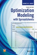
Then the objective function—the total number of patrols—can be expressed as the sum of the yj values. In the model of Figure 6.12, this sum is represented as the SUMPRODUCT of the decision row and a row containing all 1’s. To formulate constraints, we focus on row i in the array, which corresponds to sector i. The SUMPRODUCT of this row and the decisions yields the number of patrols that can service county i. In the problem, we require coverage from at least one patrol for every row. In words, our model takes the following form:

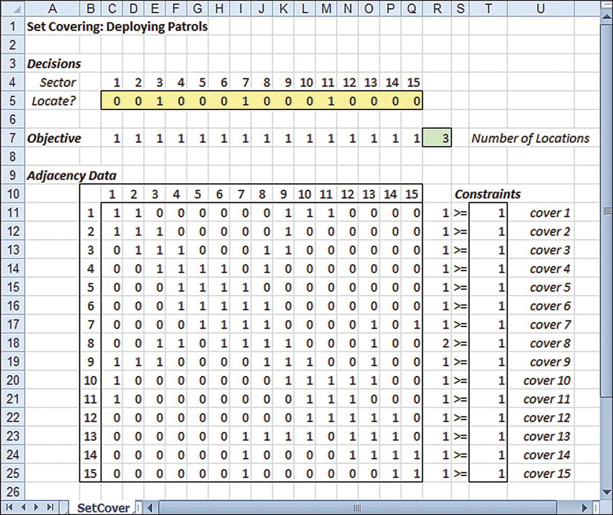
Figure 6.12 Optimal solution for Example 6.3.
In algebraic terms, we can let aij represent the adjacency data in the array of Figure 6.11. That is, aij = 1 if sectors i and j are adjacent and aij = 0 if not. Then we can write

In the spreadsheet of Figure 6.12, we have positioned the constraint information immediately to the right of the data array because the rows of the array give rise to constraints. We then specify the model as follows:

Figure 6.12 shows an optimal solution, which assigns patrols to sectors 3, 7, and 11. (Other assignments may also be optimal.) By using an integer programming model, the police department can provide the required service while minimizing the number of patrols needed.
The generic set-covering problem involves the selection of objects to meet given coverage requirements, where selection is a matter of binary choice. Each column in the constraints of the model (refer to Fig. 6.12 as an example) corresponds to an object and the coverage it provides. When the coverage is expressed with 0’s and 1’s (the constraint coefficients in a column), we can think of the 1’s as defining a coverage set (i.e., the set of rows in which 1’s appear). Thus, the selection of objects is equivalent to the selection of sets, and the problem is to choose the minimum number of sets that will provide the required coverage. This interpretation gives rise to the name set-covering problem.
6.4 SET PACKING
As we saw in Section 6.3, the covering model of linear programming leads to an analog in binary-choice programming. In a similar fashion, the allocation model of linear programming leads to another analog. This model resembles the set-covering model, except that it contains allocation constraints rather than covering constraints. To describe how this model might arise, consider the problem faced in deploying a sales force.

Figure 6.13 Map of the target area for NSH.
Again, the raw data for this problem comes from a map, and the model will involve binary choice with the objective of maximizing population coverage. In addition, the nature of potential conflict is exhibited in the “at most one” condition that applies to active sales reps in a region. In other words, we can anticipate that the constraints of the problem should ensure that no conflicts involving two or more sales reps occur in any of the 11 regions. What element potentially creates conflicts? It is not the sales reps themselves but rather the region assignments that can be in conflict. That observation tells us that although the sales reps are the objects in the problem, it is the assignments that will be the subject of binary choice. The possible assignments are the possible pairs of regions.
For modeling purposes, it’s convenient to convert this information into a conflict array, shown in Figure 6.14 as part of the full model. In the figure, the numbered rows correspond to the regions, and the columns correspond to possible assignments. An entry of 1 appears in row i and column j if assignment j involves region i.

Figure 6.14 Optimal solution for Example 6.4.
A model for maximizing the number of nonconflicting assignments can be constructed around the conflict array by defining binary variables:

Then the objective function—the total population served—can be expressed as the SUMPRODUCT of the decision row and the population values. To formulate constraints, we focus on row i in the array, corresponding to region i. The SUMPRODUCT of this row and the decisions yields the number of assignments that occupy region i. In the problem, we require this number to be at most 1 for any region. In words, our model takes the following form:

In algebraic terms, we can let cj represent the population in region j (in thousands) and let aij represent the conflict data in the array of Figure 6.14. That is, aij = 1 if region i is occupied by assignment j and aij = 0 if not. Then we can write

In the spreadsheet of Figure 6.14, we specify the model as follows:

Figure 6.14 shows the optimal solution, which calls for choosing assignments 2, 5, and 20. One sales rep will be active in regions 1 and 3; another will be active in regions 2 and 5; and the third will be active in regions 10 and 11. By using an integer programming model, NSH can deploy its sales force without conflicts and provide direct service to the maximum possible population of 332,000 students.
The generic version of this problem involves selections of sets that avoid given conflict possibilities, with selection represented by binary choice. Each column in the constraints of the model (refer to Fig. 6.14 as an example) corresponds to a set and the conflicts it potentially generates. When the conflicts are expressed with 0’s and 1’s (by the constraint coefficients in a column), we can think of the 1’s as defining a conflict set (i.e., the set of rows in which 1’s appear). Thus, the objects of the problem are assignment pairs, and the problem is to “pack in” these objects to achieve the largest possible coverage. This interpretation gives rise to the name set-packing problem.
6.5 SET PARTITIONING
As another example of binary choice, we consider a matching problem. The term “matching” refers to identifying pairs—that is, associating one object in a population with exactly one other object in the same population. This structure differs from the assignment problem of Chapter 3, which calls for matching an object in one population, such as products, to an object in another population, such as factories. Consider the exam-scheduling problem as it arises at Oxbridge College.
It’s not necessary to fill in the entire array because of symmetry: The number of conflicts between class times Ti and Tj is the same as the number of conflicts between Tj and Ti. Although it is convenient to present the data in a half array, it can also be presented in a horizontal layout, as in the standard linear programming format. (See rows 3 and 4 of Fig. 6.15.)

Figure 6.15 Spreadsheet model for Example 6.5.
The essential decision in this problem is a binary choice for matching. The binary decision variables xij are defined as follows:

Because symmetry allows us to work with just half the conflict array, we need to define the xij variables only for i < j, which comes to 28 pairs. Then we can write the objective function as a SUMPRODUCT in the form ∑cijxij, where cij represents the number of conflicts occurring when Ti and Tj are assigned to the same exam day, and the sum is taken over all 28 potential assignments. Because the quantity cij contributes to this sum only when xij = 1, the objective function measures the total number of conflicts in the exam schedule. Constraints are needed to make sure that each class time is assigned exactly one match. The algebraic model takes the following form:

Figure 6.15 shows the spreadsheet model. The layout follows the standard linear programming layout introduced in Chapter 2. By transforming the conflict data from the original half array into one long row in Figure 6.15, we facilitate the use of a standard layout.
The model specification is the following:

After running Solver, we find that the minimal number of conflicts is 76, as shown in the figure, and the optimal pairings are T1 with T5, T2 with T6, T3 with T8, and T4 with T7. By using an integer programming model, Oxbridge can thus limit the number of exam conflicts to the minimum possible level.
The binary-choice model in Figure 6.15 resembles the set-covering model except for the constraint type. Again, we can think of columns as sets, and in this case, the 1’s in each column identify the pair of class times in the corresponding match. The problem involves choosing a full match—that is, a collection of pairs such that each class time appears exactly once in the collection. The “exactly once” requirement means that the sets selected must partition the population of class times into mutually exclusive and exhaustive subsets. For that reason, this problem type is often called a set-partitioning problem.
In Example 6.5, the number of class times is exactly equal to twice the number of exam days. More generally, the number of class times could be slightly less than twice the number of exam days, and a similar model could be used. For example, if there were six class times rather than eight, we could proceed by creating two fictitious class times for which no conflicts exist. We could then solve a set-partitioning problem containing six actual and two fictitious class times. Class times that appear in that solution paired with a fictitious class time would then be interpreted as being assigned to a time period exclusively.
Although Example 6.5 arises in the setting of scheduling exams, the same kind of matching model can be used to schedule class meetings (or training courses, or conference sessions, etc.) when at most two items are scheduled per time period. Several additional conditions may apply as well, but the basic structure of such problems often corresponds to the matching problem.
When we compare the set-covering model and the set-partitioning model in our two examples, we note that they differ in the type of constraints that appear. In set covering, we selected sets to provide at least a minimum coverage, and those sets belonged to the objects in the problem (sectors). In set partitioning, we selected sets to provide exact coverage, but the sets belonged not to objects but rather to pairs of objects (matches). Thus, building a good model for binary choice requires that we recognize how sets interact, either complementing each other or conflicting with each other. In Example 6.3, the sets that complement each other and provide the desired coverage were associated with the objects of the problem. This insight associates the objects with binary choice. In Example 6.5, the sets that compete with each other to provide mutually exclusive and exhaustive coverage of courses were associated with pairs of the objects in the problem. This insight associates the assignments with binary choice.
6.6 PLAYOFF SCHEDULING
An application area for integer programming that has received increasing attention lately is the scheduling of sports teams in professional leagues. Although basic guidelines exist for the creation of a “balanced” schedule, a good deal of flexibility remains, and several specific considerations come into play in determining an “optimal” schedule. As an example, a relatively new league in Latin America has just begun to examine the possibility of optimized scheduling.
When we examine the LASA problem closely, we can identify two basic constraints: (i) Each team must play every other team, and (ii) each team plays exactly one game each week. As a consequence, the schedule must require at least 5 weeks. When we turn to the objective, we observe that each team plays two intradivision rivals. Therefore, at best, the intradivision rivalries can be placed in the last two weeks of the schedule. Normally, it is not too difficult to devise a 5-week schedule containing the 15 required games, even with pencil and paper. However, it may not be so easy to determine whether all intradivision rivalries can be placed in the last 2 (or even 3) weeks. That’s where an integer programming model can be useful.
To build the model, we rely on a binary-choice variable:

We need to define these xjkt variables for the 15 distinct pairs of teams corresponding to j < k, as well as for each of the 5 weeks. This specification gives us a total of 75 binary variables. Then it is straightforward to write the constraints of the problem. For the one-game-per-week constraints, we write

For the play-everyone-else constraints, we write

The model contains 30 constraints of type (6.1) and 15 constraints of type (6.2), for a total of 45 constraints.
For the objective function, let’s assume we wish to maximize the following expression:

This expression represents a sum containing 75 terms. In selecting the coefficients cjkt, we first need a mechanism that favors intradivision games over the other games. An easy way is to associate a zero coefficient with each pairing of teams from different divisions. Then, for the intradivision games, we need a mechanism that favors later weeks over earlier weeks. For this purpose, we could associate a positive objective function coefficient equal to the week number for each variable. Thus, we define the following coefficients:

Perhaps the notion of “later week” deserves a closer look. In our assignment of coefficient values, we would permit the model to place two intradivision games in week 4 (making a contribution of 8 to the objective) rather than placing one intradivision game in week 5 (making a contribution of just 5). However, if we do not find that trade-off desirable, we could use an alternative scheme.
The spreadsheet model for the LASA problem is not difficult to build, but we must keep its size in mind: 45 constraints and 75 variables. For reasons of readability, Figure 6.16 shows just the upper left portion of the model. The variables appear in row 15, with rows 13 and 14 containing labels for the variables. Specifically, the pair (j, k) appears in row 13, and the week t appears in row 14. The first set of constraints, corresponding to (6.1) appears in rows 18–47, and the second set, corresponding to (6.2) appears in rows 49–63. Row 48 reproduces the team pair in row 13 for easier reference.

Figure 6.16 Portion of the spreadsheet model for Example 6.6.
Figure 6.17 shows the entire model. All the constraints are equations with right hand-side constants equal to 1, so this model takes the form of a set-partitioning problem. The sets of constraints corresponding to (6.1) and (6.2) each have distinctive, repeating clusters of nonzero coefficients, which become visible when we zoom out and display the entire model in one window. By examining the model at this zoom level, we can scan the layout for possible typos or omissions.

Figure 6.17 Spreadsheet model for Example 6.6.
The model specification is the following:

A solution appears in both Figures 6.14 and 6.15, but the entire schedule is more usefully displayed in a table such as in Table 6.1, with shading to designate intradivision games.
Table 6.1 Playoff Schedule for LASA
| Week | ||||||
| 1 | 2 | 3 | 4 | 5 | ||
| Team | 1 | 16 | 15 | 12 | 13 | 14 |
| 2 | 24 | 26 | 21 | 25 | 23 | |
| 3 | 35 | 34 | 36 | 31 | 32 | |
| 4 | 42 | 43 | 45 | 46 | 41 | |
| 5 | 53 | 51 | 54 | 52 | 56 | |
| 6 | 61 | 62 | 63 | 64 | 65 | |
In the optimal schedule, all intradivision games are played in weeks 3–5. Although six intradivision games must be played, they cannot all fit into the final two weeks of the schedule.
The LASA scenario leads to a simple version of the playoff scheduling problem. In actual practice, administrative bodies are concerned about several other features of a schedule. For example, it’s common to keep track of home and away games and to restrict a schedule so that no team plays more than two consecutive games at home. In other settings, governing boards keep track of especially “strong” teams and require that no team be scheduled to play two strong teams in successive weeks. Finally, in many countries, soccer games compete with cultural events, so leagues often prohibit games on dates corresponding to local festivals, bicycle races, or religious celebrations. Considerations such as these can be accommodated with integer programming models, but sometimes the scheduling models grow quite large.
6.7 THE ALGORITHM FOR SOLVING INTEGER PROGRAMS
We can give a rough outline of the procedure that Solver uses to find solutions to integer programming models, drawing on an example. For this purpose, we revisit Example 2.1 (Brown Furniture Company), in which the problem is to determine the best allocation of resources to the production of chairs, desks, and tables. Suppose the problem has changed slightly so that there are 1900 available hours of fabrication capacity, 1850 of machining, and 1450 of assembly, along with 9600 sq. ft of wood. The linear programming problem is as follows:

Now we require all variables in the solution to be integers—that is, we want the number of chairs, desks, and tables to all be integers so that we can interpret the solution literally, as a viable schedule for the month.
When Solver tackles an integer programming problem, its first step is simply to ignore the integer restrictions and treat the problem as a normal linear program. This is called the relaxed problem, in the sense that the integer constraints are relaxed. We denote this linear program as problem P. If we are fortunate, the optimal solution for the relaxed problem will contain integer decision variables, and it will give us the solution we seek. In this example, unfortunately, the optimal solution does not consist of integers, and we obtain

The value of the objective function is at least an upper bound on the best value we could attain with integer values. No integer-valued solution could improve on the solution to the relaxed problem, in which the integer constraints do not apply.
Solver recognizes that this solution is infeasible for the integer program and creates two new linear programming problems to solve. The first, which we denote as P1, corresponds to problem P, with the additional constraint D ≤ 227. The second, denoted P2, corresponds to problem P, with the requirement D ≥ 228 instead. In other words, we select a noninteger variable in the optimal solution and append one of two constraints: We force this variable to be either no larger than the next lower integer or no smaller than the next higher integer. We could use an arbitrary rule to select which variable to constrain or a rule with a little more intelligence. Here, we choose the variable that is closest to an integer value, which is the variable D.
The better of the solutions to the integer versions of P1 and P2 must be the optimal solution to the original problem. The reason is that together the two problems correspond to all feasible choices of integer decision variables because they exclude only the cases associated with D values strictly between 227 and 228, none of which is an integer. The implication is that we can forget the original problem for now and concentrate just on the two modified problems that replaced it, P1 and P2. If we can solve both of those as integer programs (and then choose the better of the two solutions), we will have the optimal solution to the original problem.
Next, Solver tackles P1. Intuitively, we might expect the optimal solution to contain D at its ceiling of 227 because it “wants” to be 227.8, but the additional constraint prevents it from being so large. Indeed, that is the case, and we obtain the following result:
As we might expect, the additional constraint leads to a drop in the optimal objective function. More importantly, we still weren’t lucky enough to produce an integer solution because C remains noninteger.
When Solver tackles P2 (where D ≥ 228), the optimal solution is as follows:

Having replaced the original problem with two modified problems, the status of our search is shown in Figure 6.18. Here, each (linear programming) problem is represented by a node in the tree diagram. We say that we branch from the original problem P to the modified problems P1 and P2. This means that we need only examine the two replacement problems and not the original. In a sense, the search has been effective so far because we started with a model that generated two noninteger decision variables, but now, we are dealing with models that generate only one noninteger decision variable.

Figure 6.18 First level of branching.
Next, we select P1 for branching. We recognize that the optimal solution is infeasible for the integer version of P1 because the value of C is noninteger. Hence, we create two modified versions to solve, one in which we add the constraint C ≤ 9; the other in which we add the constraint C ≥ 10. These bounds use the integers on either side of the value of C in the optimal solution to P1. We refer to these problems as P11 (with C ≤ 9) and P12 (with C ≥ 10). Now we can forget P1. The best among the integer solutions of P11, P12, and P2 will be the solution we seek.
When we solve P11, we obtain the following result:

The optimal solution is still noninteger, and the objective function has dropped slightly from the value in P1. When we solve P12, we obtain the following result:

Here, we have been fortunate, and the solution to the linear program contains three integer-valued decision variables. It was not merely good fortune, of course: The systematic choice of additional constraints helped lead us to an integer solution. This solution is a feasible integer solution to the original problem. Now, the status of our search is shown in Figure 6.19. In principle, we could pursue the search from P11 or P2.

Figure 6.19 Second level of branching.
Consider the linear program in P2 and its objective function, which Solver has optimized at 4698.7. The solution of P2 is still not feasible for the integer program, and the only way we can produce an integer-feasible solution is to impose additional constraints. Thus, the value 4698.7 represents an upper bound on the best solution we could find in this part of the search tree. When we add constraints to P2, its objective function cannot get better, so it can be no larger than 4698.7. Since we have already found an integer-feasible solution with an objective function value of 4700, there is no reason to look for a feasible solution to P2 because its objective function value could not be as good as the 4700 we have already found. We say that we have fathomed the search tree below P2, in the sense that we have implicitly evaluated all the branches that might emanate from P2 and determined from the bound that none of the branches could be as good as the feasible solution we have already encountered.
We turn next to P11. Its bound is 4700.3. Because this value is larger than that of the best integer solution we have found, it is still possible that we could find a better solution by branching from P11. Because the only noninteger decision variable in P11 is T = 1.17, we branch to P111 (adding the constraint T ≤ 1) and P112 (adding the constraint T ≥ 2), and we obtain the following results:


We now have enough information to identify the optimal solution to the original problem. The solution to P111 contains integer decision variables, but its objective function is not as large as the integer-feasible solution to P12. In addition, we can fathom P112 because its upper bound is 4699.5, also not as large as the integer-feasible solution to P12. The final status of our search is shown in Figure 6.20, where we can see that the solution to P12 turns out to be optimal.

Figure 6.20 Final status of tree search.
For any integer linear programming problem, Solver begins with the relaxed problem and finds the optimal solution to the corresponding linear program. If all of the variables are integer, the solution to the integer program has been found. If not, x1 will turn out to be either an integer or a fraction. If it is a fraction, Solver replaces the original problem with two derived problems (P1 and P2), each with an additional constraint that forces the solution away from the fractional value in the original. On the other hand, if x1 is an integer, Solver then examines x2. Two alternatives may arise, depending on whether x2 is an integer or a fraction. If it is a fraction, Solver creates two derived problems containing additional constraints that force the solution away from the fractional value of x2. Otherwise, Solver proceeds to examine x3 and so on.
At each stage in this procedure, Solver maintains a list of unsolved problems. This list is structured so that the best integer-feasible solution to the problems on the list will be the optimal solution for the original model. One at a time, problems are removed from the list and addressed by solving them as linear programs. Either the solution will be integer-feasible, or the problem will be replaced by two other problems, each containing an additional constraint. This procedure requires the solution of a series of linear programs. The list might get quite long, but the procedure ultimately produces an optimal solution with integer-valued decision variables. The replacement of a problem on the list by two others is called branching. This name comes from a tree-like diagram that traces the different problems (as in Fig. 6.20).
As we saw, it is possible to curtail the list of problems that remain to be solved. Any time we encounter an integer-feasible solution, the branching in that portion of the tree is finished. Elsewhere, branching may lead to an infeasible linear program, which also terminates branching. Otherwise, we can try to use the bounds to fathom certain problems and also terminate branching in part of the search tree. Suppose that, at some stage of solving a maximization problem, the list contains a problem with a value (upper bound) that is worse than the value of the objective function in an integer-feasible solution already encountered. Whenever the bound on a derived problem is worse than the value of a known integer solution, then the derived problem may be removed from the list because its solution could never be optimal. (The mirror image of this statement holds when we are minimizing; in that case, whenever the bound on a derived problem is higher than the value of a known integer solution, we can remove the derived problem from the list.)
The generic name for the overall procedure Solver uses is branch and bound, reflecting the two mechanisms that guide the search. Branching replaces a problem on the list with two problems that are, in some sense, closer to being solved as integer programs. Bounding explores whether a particular problem could just be deleted from the list because it offers no hope of finding an optimum. Nevertheless, the essence of the procedure is to solve a number of linear programs, to replace one problem with two whenever an integer constraint is violated, and to use bounds to remove problems from the list in order to reduce the workload. Because this procedure relies on the solution of many linear programs, it is as reliable a procedure as the linear solver on which it depends. That is, the branch-and-bound procedure is guaranteed to produce an optimal solution.
SUMMARY
The ability to treat variables as integer valued, and in particular, the ability to designate variables as binary, opens up a wide variety of optimization models that can be addressed with Solver. This chapter introduced two broad classes of models that can be handled effectively with Solver. The first type of model is one that resembles a linear program but with the requirement that certain variables must be integer valued. For the purposes of using Solver, this requirement is added to the linear programming model as an additional constraint. The second type of model is one in which certain decisions exhibit an all-or-nothing structure, representing actions that are indivisible. Such decisions are modeled by binary variables, which are simply integer-valued variables no less than 0 and no greater than 1. Binary variables allow us to model the occurrence of yes/no choices and to exploit Solver, provided that the structure of the model is linear in all other respects.
In this second category, we explored three closely related model structures: set covering, set packing, and set partitioning. In the basic form of these models, the objective function coefficients and the right hand-side constants are 1’s, but generalizations are also possible, as illustrated in some of the exercises at the end of this chapter.
In the next chapter, we examine a broader set of integer programming models based on the ability to represent logical constraints using binary variables. In those models, the logical conditions do not seem linear, but they can be expressed in linear forms with the help of binary variables.
EXERCISES
- 6.1 Callum Communications (Revisited): Revisit Example 6.1. Suppose that the objective at Callum Communications is to minimize the number of employees, rather than to minimize the total cost.
- What is the minimum number of employees needed at the call center?
- Does the solution in (a) achieve the minimum salary cost?
- 6.2 Make or Buy: A sudden increase in the demand for smoke detectors has left Acme Alarms with insufficient capacity to meet demand. The company has seen monthly demand from its retailers for its electronic and battery-operated detectors rise to 20,000 and 10,000, respectively, and Acme wishes to continue meeting demand. Acme’s production process involves three departments: Fabrication, Assembly, and Shipping. The relevant quantitative data on production and prices are summarized below.
Department Monthly Hours Available Hours/Unit(Electronic) Hours/Unit(Battery) Fabrication 2000 0.15 0.10 Assembly 4200 0.20 0.20 Shipping 2500 0.10 0.15 Variable cost/unit $18.80 $16.00 Retail price $29.50 $28.00 - The company also has the option to obtain additional units from a subcontractor, who has offered to supply up to 20,000 units per month in any combination of electronic and battery-operated models, at a charge of $21.50 per unit. For this price, the subcontractor will test and ship its models directly to the retailers without using Acme’s production process.
- Acme wants an implementable schedule, so all quantities must be integers. What are the maximum profit and the corresponding make/buy levels?
- Compare the maximum profit in (a) to the maximum profit achievable without integer constraints. Does the integer solution correspond to the rounded-off values of the noninteger solution? By how much (in percentage terms) do the integer restrictions alter the value of the optimal objective function?
- 6.3 Selecting an Investment Portfolio: An investment manager wants to determine an optimal portfolio for a wealthy client. The fund has $2.5 million to invest, and its objective is to maximize total dollar return from both growth and dividends over the course of the coming year. The client has researched eight high-tech companies and wants the portfolio to consist of shares in these firms only. Three of the firms (S1–S3) are primarily software companies, three (H1–H3) are primarily hardware companies, and two (C1–C2) are Internet consulting companies. The client has stipulated that no more than 40% of the investment be allocated to any one of these three sectors. To ensure diversification, at least $100,000 must be invested in each of the eight stocks. Moreover, the number of shares invested in any stock must be a multiple of 1000.
- The table below gives estimates from the investment company’s database relating to these stocks. These estimates include the price per share, the projected annual growth rate in the share price, and the anticipated annual dividend payment per share.
Stock S1 S2 S3 H1 H2 H3 C1 C2 Price per share $40 $50 $80 $60 $45 $60 $30 $25 Growth rate 0.05 0.10 0.03 0.04 0.07 0.15 0.22 0.25 Dividend $2.00 $1.50 $3.50 $3.00 $2.00 $1.00 $1.80 $0.00 - Determine the maximum return on the portfolio. What is the optimal number of shares to buy for each of the stocks? What is the corresponding dollar amount invested in each stock?
- Compare the solution in which there is no integer restriction on the number of shares invested. By how much (in percentage terms) do the integer restrictions alter the value of the optimal objective function? By how much (in percentage terms) do they alter the optimal investment quantities?
- 6.4 Selecting New Products: A video game company has an R&D group with 30 programmers. The group has been given a budget of $1 million for this year to develop and test new game designs for introduction next year. The new games have been outlined, each with the ancillary expenses that will be incurred and the number of programmers that will be needed. A panel of marketing specialists has estimated the potential revenues from each game. The problem for the R&D group is to generate the maximum level of potential revenues from its limited expense budget and its available programmers. What is the maximum level?
Game 1 2 3 4 5 6 7 8 Revenue 325 275 320 220 190 265 360 285 Expense 200 130 240 120 115 135 105 280 Programmers 6 5 8 4 5 5 7 6 - 6.5 Choosing R&D Projects: Texas Electronics Company (TEC) is contemplating a research and development program encompassing eight major projects. The company is constrained from embarking on all of the projects by the number of available scientists (40) and the budget available for projects ($300,000). In the following are the resource requirements and the estimated profit for each project.
Project Expense ($000) Scientists Required Profit ($000) 1 60 7 36 2 110 9 82 3 53 8 29 4 47 4 16 5 92 7 56 6 85 6 61 7 73 8 48 8 65 5 41 - What is the maximum profit, and which projects should be selected?
- Suppose that projects 2 and 5 are mutually exclusive. That is, TEC should not undertake both. As a result, what is the revised project portfolio and the revised maximum profit?
- In addition, suppose that projects 5–8 involve consumer products and that management decides to undertake at least two of those. As a result, what is the revised project portfolio and the revised maximum profit?
- 6.6 Stocking Warehouses: Nicklaus Razor Blade (NRB) Company plans to test market a new blade next month. The blades will be stocked in their three warehouses in the following quantities.
Warehouse A B C Stock (cartons) 50 50 50 - The carton quantities required by the distributors in the four test markets are as follows.
Distributor D E F G Requirement 45 15 25 20 - The unit costs (in dollars per carton) of shipping the blades from warehouses to distributors are given in the table below.
D E F G A 8 10 6 3 B 9 15 8 6 C 5 12 5 7 - If the NRB Company wishes to meet the distributor’s requirements at the minimum total transportation cost, what is the optimal distribution plan and its cost?
- Suppose that the policy at the NRB Company is that each distributor must be serviced by a single warehouse. What is the optimal distribution plan under this policy?
- By how much (in percentage terms) does the single-warehouse policy inflate distribution cost?
- 6.7 Reservation Scheduling: Roth Auto Rentals, a car rental company specializing is SUVs, is making up a schedule for the next weekend’s demands. The peak demand period occurs on the weekend, when Roth may not have enough SUVs to meet demand. The customer demands that have been logged in are listed below.
Days Customers Friday–Monday 1 Friday–Saturday 4 Friday–Sunday 5 Saturday–Sunday 4 Saturday–Monday 3 Sunday–Sunday 2 - The rental cost depends on which days the contract covers, as shown in the next table.
Days FSSM FS FSS SS SSM Sunday Rate 119.95 69.95 99.95 74.95 89.95 39.95 - Roth Auto Rentals carries only one type of vehicle and expects to have 10 SUVs available for rental over the weekend.
- What is the maximum revenue that can be generated from the list of orders?
- In the optimal solution of (a), what percentage of customer demand is satisfied?
- In the optimal solution of (a), what percentage of dollar demand is satisfied?
- Answer the set of three questions above for fleet sizes of 11–16.
- 6.8 Allocating Components to Assemblies: Biking.com is a web-based company that sells bicycles on the Internet. Its distinctive feature is that it allows customers to customize the design when they order and then to receive quick delivery. Biking.com gives customers choices for frame size (34, 36, 38), suspension (standard or heavy-duty), and gear speeds (5, 10, 15). As a result, customers can order one of 18 possible combinations (3 × 2 × 3). The company shorthand refers to frame size as Option A (A1 is the 34-in. model, A2 is the 36-in. model, and A3 is the 38-in. model). Similarly, the standard suspension is option B1, and the heavy-duty suspension is B2. The gear speeds are C1 (5), C2 (10), and C3 (15). Rather than stock 18 different types of bicycles, the company holds inventories of the major components and then assembles the bikes once a customer order comes in. Orders are taken Mondays through Wednesdays, assemblies are done on Thursdays, and shipments go out on Fridays. Thus, at the close of business on Wednesday, the company has an inventory of components and a list of orders, and its task is to match components with orders to meet as much demand as possible. The tables below describe customer orders for this week and the inventory status at the end of Wednesday.
Model 1 2 3 4 5 6 7 8 9 10 11 12 13 14 15 16 17 18 A 1 1 1 1 1 1 2 2 2 2 2 2 3 3 3 3 3 3 B 1 1 1 2 2 2 1 1 1 2 2 2 1 1 1 2 2 2 C 1 2 3 1 2 3 1 2 3 1 2 3 1 2 3 1 2 3 Orders 4 5 0 5 1 7 0 4 8 1 2 0 5 6 4 0 1 5 Component A1 A2 A3 B1 B2 C1 C2 C3 Inventory 12 20 30 20 25 18 16 20 - What is the maximum number of customer orders that can be satisfied this week?
- Suppose that the profitability varies by model type, as shown in the table below. What is the maximum profit that can be achieved from this week’s orders?
Model 1 2 3 4 5 6 7 8 9 10 11 12 13 14 15 16 17 18 Profit 45 55 70 65 75 90 47 57 72 67 77 92 50 60 75 70 80 95 - 6.9 The Latin American Soccer Association (Revisited): Revisit Example 6.6. Suppose that the Latin American Soccer Association (LASA) decides to create a longer playoff schedule. They want each team to play two games against the teams in its own division and one game against each team in the other division. Construct a playoff schedule that maximizes the number of games played by intradivision rivals toward the end of the season.
- How many weeks are required for the entire schedule?
- How many variables and constraints appear in the optimization model?
- What is an optimal schedule for LASA?
- Review your schedule in part (c) and determine whether the same two teams ever meet in successive weeks. Amend the model to prohibit such meetings and construct an optimal schedule.
- 6.10 One-Dimensional Cutting Stock Problem: Lumber is supplied to a medium-sized furniture workshop in standard lengths of 100 in. Different designs call for pieces of specified lengths that do not exceed 100 in. Nevertheless, the shop wants to use a minimum number of standard-length master pieces to accommodate a given list of required pieces. Today’s list is shown in the table below.
Design 1 2 3 4 5 6 7 8 9 10 11 Length 33 14 63 84 39 94 54 41 50 71 56 - Develop a rule of thumb to solve this problem. How many standard-length pieces are needed, using your rule of thumb?
- What is the optimal solution? How close did your rule of thumb in (a) come to the optimum?