
Chapter 6
Endogeneity
6.1 Introduction
There is an endogeneity problem when the error is correlated with at least one explanatory variable. This phenomenon is very common in econometrics because, compared to experimental sciences, it is not possible (or it is at least difficult) to control the data‐generating process. Among the possible causes of endogeneity, the three most important are:
- simultaneity. In this case, there is an explanatory variable that is set simultaneously with the response: this is, for example, the case when one seeks to estimate a demand equation for a good, which contains the price of the good itself. The demand and the price are simultaneously set by the condition of equality of supply and demand and, therefore, a variation of the error term of the demand equation will shift the demand curve and therefore induce a variation of the quantity and the equilibrium price. The price variable is therefore endogenous.
- covariate measured with error. If the “true” model is
 and what is observed is
  , the estimated model writes:
  , or
, or 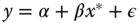 with
with  . Hence,
  is correlated with
  , which is therefore endogenous.
 - omitted variable. If the “true” model is
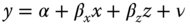 and
and  is unobserved, the estimated model is
 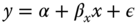 , with
  . The error of the estimated model then contains the influence of the omitted variable, and this error is correlated with
  if
if  and
and  are correlated. Once again, the covariate
  is then endogenous.
The OLS estimator is:
Replacing ![]() by its expression:
by its expression: ![]() , we obtain
, we obtain ![]() as a function of the errors of the model:
as a function of the errors of the model:
We then have, denoting ![]() the sample size:
the sample size:
The estimator is consistent (![]() ) if
) if ![]() , this expression being the vector of covariances for the population between the covariates and the error. The ordinary least squares model is therefore consistent if the covariates and the error are uncorrelated. When this condition is not met, the method of instrumental variables, which will be presented in detail in this chapter, can be used.
, this expression being the vector of covariances for the population between the covariates and the error. The ordinary least squares model is therefore consistent if the covariates and the error are uncorrelated. When this condition is not met, the method of instrumental variables, which will be presented in detail in this chapter, can be used.
Concerning simultaneity, there is an additional problem as the model is not defined by one equation but by a system of equations. In this case, two strategies can be followed:
- estimating only the equation of interest (limited information estimator),
- estimating simultaneously all the equations (full information estimator).
The latter approach leads to a more efficient estimator, as the correlation of the errors of all the equations is taken into account. But if an equation is wrongly specified, it can contaminate the estimation of the parameters of the other equations of the model.
6.2 The Instrumental Variables Estimator
6.2.1 Generalities about the Instrumental Variables Estimator
Let us consider the following model: ![]() with
with ![]() . if at least one of the covariates is correlated with the errors, the OLS estimator is not consistent. In order to obtain consistency, we use the instrumental variables estimator. The instrumental variables are denoted by
. if at least one of the covariates is correlated with the errors, the OLS estimator is not consistent. In order to obtain consistency, we use the instrumental variables estimator. The instrumental variables are denoted by ![]() .1 Denoting by
.1 Denoting by ![]() the number of the covariates and by
the number of the covariates and by ![]() the number of instruments (not including the column of ones), the instrumental variables must verify:
the number of instruments (not including the column of ones), the instrumental variables must verify: ![]() . Stated differently, they must not be correlated with the errors.2 In the simplest case where the number of instruments equals the number of covariates, the instrumental variable estimator is simply obtained by solving the system of equations:
. Stated differently, they must not be correlated with the errors.2 In the simplest case where the number of instruments equals the number of covariates, the instrumental variable estimator is simply obtained by solving the system of equations: ![]() , which is just identified. Developing this expression, we obtain:
, which is just identified. Developing this expression, we obtain: ![]() , which can also be written:
, which can also be written:
If there are more instruments than covariates (![]() ),
), ![]() is an over‐determined system of linear equations, which, except for very special cases, doesn't have a solution. In this case, two equivalent approaches can be used to obtain the optimal estimator. The first one consists in pre‐multiplying the model by
is an over‐determined system of linear equations, which, except for very special cases, doesn't have a solution. In this case, two equivalent approaches can be used to obtain the optimal estimator. The first one consists in pre‐multiplying the model by ![]() :
:
It is a model that contains ![]() rows and
rows and ![]() parameters to estimate
parameters to estimate ![]() . If one considers it as a standard regression model, the variance of the errors being
. If one considers it as a standard regression model, the variance of the errors being ![]() , the best linear estimator is the GLS estimator, and we then obtain the following instrumental variables estimator:
, the best linear estimator is the GLS estimator, and we then obtain the following instrumental variables estimator:
with ![]() .
.
The second approach is the generalized method of moments. We consider here a vector of ![]() moments:
moments: ![]() for which the variance is
for which the variance is ![]() . Using the generalized method of moments, we seek to minimize the quadratic form of the vector of moments, using the inverse of the variance matrix of these moments:
. Using the generalized method of moments, we seek to minimize the quadratic form of the vector of moments, using the inverse of the variance matrix of these moments:
The first‐order conditions for a minimum are: ![]() , and solving this system of linear equations, we obtain the same estimator as before.
, and solving this system of linear equations, we obtain the same estimator as before.
The instrumental variables estimator is also called the two‐stage least squares estimator (2SLS), as it can be obtained by applying twice the method of ordinary least squares. When we consider the regression of ![]() on
on ![]() , we obtain the estimator
, we obtain the estimator ![]() and the fitted values
and the fitted values ![]() . The matrix
. The matrix ![]() is therefore the projection matrix on the subspace defined by the columns of
is therefore the projection matrix on the subspace defined by the columns of ![]() . This matrix is symmetric and idempotent, which means that
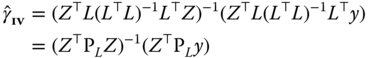
. This matrix is symmetric and idempotent, which means that ![]() . The instrumental variables estimator 6.3 can also be written, denoting by
. The instrumental variables estimator 6.3 can also be written, denoting by ![]() the fitted values of the covariates regressed on the instrumental variables:
the fitted values of the covariates regressed on the instrumental variables:
and can therefore be obtained by applying OLS twice:
- the first time by regressing every covariate on the instruments,
- the second time by regressing the response on the fitted values of the first‐stage estimation.
The variance of the instrumental variables estimator is:
The estimator is therefore the more efficient the larger the variance of ![]() , which means that
, which means that ![]() and
and ![]() are highly correlated.
are highly correlated.
6.2.2 The within Instrumental Variables Estimator
The specificity of panel data methods is that the error term is modeled as having two components, an individual effect and an idiosyncratic term. Therefore, the correlation between covariates and instrumental variables, on the one hand, and the errors of the model, on the other hand, must be analyzed separately for each component of the error. In this section, we consider the estimation of the model transformed in deviations from individual means. This transformation wipes out the individual effect; therefore, there is no reason to take care of the correlation between the covariates and the individual effects. The ![]() is obtained by pre‐multiplying the model first by
is obtained by pre‐multiplying the model first by ![]() :
: ![]() and then by
and then by ![]() ,
,
and applying GLS to this transformed data, the variance matrix of the errors of this model being ![]() :
:
or, denoting by: ![]() the projection matrix defined by the within transformation of the instruments:
the projection matrix defined by the within transformation of the instruments:
A similar reasoning can be followed for the between model. We consider the between transformation of the model ![]() , with the same transformation applied to the instruments (
, with the same transformation applied to the instruments (![]() ). The instrumental variables estimator is obtained by pre‐multiplying the model by
). The instrumental variables estimator is obtained by pre‐multiplying the model by ![]() :
:
and applying to this transformed model the GLS estimator:
with ![]() .
.
The ![]() is consistent, even if the individual effects are correlated with the covariates. On the contrary, the
is consistent, even if the individual effects are correlated with the covariates. On the contrary, the ![]() is consistent only if there is no correlation. If this hypothesis is verified, none of them is efficient, as each of them take into account only one component of variability.
is consistent only if there is no correlation. If this hypothesis is verified, none of them is efficient, as each of them take into account only one component of variability.
6.3 Error Components Instrumental Variables Estimator
In the previous section, the potential correlation between some covariates and the individual effects has been treated drastically by using the within transformation, which wipes out the individual effects. In this section, we present the error component instrumental variables estimator. The two components of the error being present in this model, it is in this case essential to tackle the issue of a potential correlation of some covariates with the two components of the error.
6.3.1 The General Model
Suppose in a first step that the idiosyncratic component of the error is not correlated with the covariates. In this case, if all the covariates are uncorrelated with the individual effects, the unbiased efficient estimator is the GLS estimator. This estimator enables, on the one hand, to take into account part of the inter‐individual variation in the sample and, on the other hand, to estimate parameters associated with covariates that don't exhibit temporal variations.
If, on the contrary, all the covariates are correlated with the individual effects, Mundlak (1978) (see subsection 4.2) has shown that the efficient estimator, which is the GLS estimator, is the same as the within estimator if the correlation between the individual effects and the covariates (more precisely the individual means of the covariates) is taken into account.
When only some covariates are correlated with the individual effects, none of the two previous estimators is appropriate any more:
- the GLS estimator is not consistent anymore because of the correlation of some covariates with the individual effects,
- the within estimator is still consistent but not efficient any more, as it doesn't take into account the fact that some covariates are uncorrelated with the individual effects but wipes out all the inter‐individual variation in the sample, especially the covariates that don't exhibit any temporal variation.
The best solution in this case consists then in using an estimator that, on the one hand, uses instrumental variables and, on the other hand, exploits the two sources of variability of the panel in an optimal way. The essential question is then to find good instruments, which is often a difficult task. The richness of panel data allows to overcome this problem. Actually, every covariate can generate two instrumental variables, using the between and the within transformations. If a rank condition that will be detailed later on is checked, the model can then be estimated without any external instrument. This approach has been used by Hausman and Taylor (1981), Amemiya and MaCurdy (1986), and Breusch et al. (1989).
If, from now, we suspect that some covariates are also correlated with the idiosyncratic part of the error, then none of the estimators we have listed above is consistent. We then use an instrumental variables estimator (within or GLS) using external instruments. This strategy has been developed by Baltagi (1981) with his “error component two‐stage least squares” ![]() estimator and by Balestra and Varadharajan‐Krishnakumar (1987) with their “generalized two‐ stage least squares”
estimator and by Balestra and Varadharajan‐Krishnakumar (1987) with their “generalized two‐ stage least squares” ![]() estimator, which differ by the way the instruments are introduced in the model.
estimator, which differ by the way the instruments are introduced in the model.
This two branches of the literature have been developed separately, and this dichotomy exists also in most software packages, which usually provide two different functions to estimate these models. We'll follow the approach of Cornwell et al. (1992), who provide a unified view of panel models with instrumental variables. These authors consider three kinds of variables:
- the endogenous variables, which are correlated with the two components of the error,
- the simply exogenous variables, which are correlated with the individual effects but not with the idiosyncratic part of the error,
- the doubly exogenous variables, which are uncorrelated with both components of the error.
Variables from the first category don't provide any usable instrument. For the second one, the within transformation is a valid instrument, as it is by construction orthogonal to the individual effects and by hypothesis uncorrelated with the idiosyncratic part. Finally, each covariate of the third category provides two instruments by using the within and the between transformation.
Consider now the specific case of time‐invariant covariates. For these variables, ![]() and
and ![]() . Therefore, such a variable provides either one instrument, if it is uncorrelated with the individual effects (the covariate itself), or no instrument.
. Therefore, such a variable provides either one instrument, if it is uncorrelated with the individual effects (the covariate itself), or no instrument.
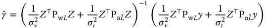
We start with the model to be estimated written in matrix form:
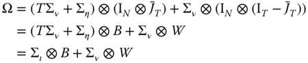
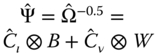
With the usual hypotheses concerning the error component model, the variance matrix of the error is: ![]() . We first pre‐multiply the model by:
. We first pre‐multiply the model by: ![]() and then obtain a transformed model for which the errors are iid.
and then obtain a transformed model for which the errors are iid.
We then apply to this model the instrumental variables method, using a set of instruments, which, denoting by ![]() the doubly exogenous variables, by
the doubly exogenous variables, by ![]() the simply exogenous variables, and by
the simply exogenous variables, and by ![]() the whole set of instruments, can be written:
the whole set of instruments, can be written:
where ![]() is a set of variables that will be defined later. For now, just consider that these variables must provide valid instruments when the between transformation is applied.
is a set of variables that will be defined later. For now, just consider that these variables must provide valid instruments when the between transformation is applied.
The instrumental variables estimator is, denoting by ![]() the projection matrix defined by the instruments:
the projection matrix defined by the instruments:
The two matrices ![]() and
and ![]() being orthogonal, the projection matrix may also be written as the sum of two projection matrices defined by the instruments transformed by the within and the between matrices:
being orthogonal, the projection matrix may also be written as the sum of two projection matrices defined by the instruments transformed by the within and the between matrices:
The estimator is then:
or also, denoting ![]() :
:
One can check that, as in the simple error component model, this estimator is a weighted average of the within and the between estimators: ![]() , with:
, with:

Several models proposed in the literature are special cases of this general model.
6.3.2 Special Cases of the General Model
6.3.2.1 The within Model
Firstly, if there are no external instruments and if all the covariates are simply exogenous, we have ![]() and
and ![]() , and the within estimator results.
, and the within estimator results.
Then, if all the covariates are either simply exogenous or endogenous and if the external instruments are simply exogenous, we also have ![]() , and
, and ![]() is constituted only by simply exogenous covariates and external instruments. The condition for identification is then that the number of external instruments must be at least equal to the number of endogenous covariates. We then have the within instrumental variables estimator:
is constituted only by simply exogenous covariates and external instruments. The condition for identification is then that the number of external instruments must be at least equal to the number of endogenous covariates. We then have the within instrumental variables estimator:
6.3.2.2 Error Components Two Stage Least Squares
Baltagi (1981)'s estimator is the special case where ![]() , which means that all the instruments (and potentially some of the covariates) are assumed to be doubly exogenous and are therefore used twice. We start from equations 6.5 and 6.7, which leads respectively to the within and between estimators. Stacking these two equations, we obtain:
, which means that all the instruments (and potentially some of the covariates) are assumed to be doubly exogenous and are therefore used twice. We start from equations 6.5 and 6.7, which leads respectively to the within and between estimators. Stacking these two equations, we obtain:

which is justified by the fact that the vector of parameters to be estimated ![]() is the same in the two equations. In order to apply GLS, we compute the variance of the errors of the stacked model:
is the same in the two equations. In order to apply GLS, we compute the variance of the errors of the stacked model:

We then apply the formula of the GLS estimator:

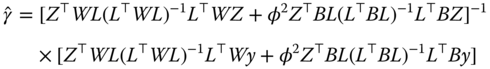
and we finally obtain:
which is the special case of the general model defined by equation 6.9 for which ![]() .
.
6.3.2.3 The Hausman and Taylor Model
In the Hausman and Taylor (1981) model, there are no endogenous variables, only simply or doubly exogenous variables. We then have ![]() ,
, ![]() and
and ![]() . Moreover, the authors stress the presence of variables with (
. Moreover, the authors stress the presence of variables with (![]() ) or without (
) or without (![]() ) time variation. The set of instruments they use is:
) time variation. The set of instruments they use is:
Only covariates that exhibit time variation may be used with their within transformation ![]() ) and doubly exogenous time‐invariant variables are used without transformation as instruments (
) and doubly exogenous time‐invariant variables are used without transformation as instruments (![]() ). Without external instruments, denoting by
). Without external instruments, denoting by ![]() the number of covariates of the 4 categories, the number of instruments is
the number of covariates of the 4 categories, the number of instruments is ![]() as the number of covariates is:
as the number of covariates is: ![]() . The model is then identified if
. The model is then identified if ![]() , i.e., if the number of doubly exogenous time‐varying variables (which provide two instruments) is greater than the number of time‐invariant simply exogenous variables, which provide no instrument.
, i.e., if the number of doubly exogenous time‐varying variables (which provide two instruments) is greater than the number of time‐invariant simply exogenous variables, which provide no instrument.
6.3.2.4 The Amemiya‐Macurdy Estimator
Hausman and Taylor (1981)'s estimator is consistent if the individual means of the doubly exogenous variables are uncorrelated with the individual effects. Amemiya and MaCurdy (1986) use the stronger hypothesis that the doubly exogenous variables are uncorrelated with the individual effects for each period. We then have: ![]() for every doubly exogenous covariate. The corresponding instrument matrix is constructed the following way. Let
for every doubly exogenous covariate. The corresponding instrument matrix is constructed the following way. Let ![]() be the matrix of doubly exogenous instruments of dimension
be the matrix of doubly exogenous instruments of dimension ![]() for individual
for individual ![]() .
. ![]() is a vector of length
is a vector of length ![]() obtained by stacking the columns of
obtained by stacking the columns of ![]() . The instrument matrix for individual
. The instrument matrix for individual ![]() is then
is then ![]() , and for the whole sample, we obtain a matrix of dimension
, and for the whole sample, we obtain a matrix of dimension ![]() :
:

6.3.2.5 The Breusch, Mizon and Schmidt's Estimator
Breusch et al. (1989) expand the instruments used by Amemiya and MaCurdy (1986) by assuming that the within transformations of simply exogenous covariates are valid instruments at every period. Stated differently: ![]() . We then obtain the further matrix of instruments
. We then obtain the further matrix of instruments ![]() by applying to
by applying to ![]() the same transformation than the one used in equation 6.11. The other contribution of Breusch et al. (1989) is to show how the different estimators can be presented in a consistent and nested way. They use the fact that the projection subspace defined by
the same transformation than the one used in equation 6.11. The other contribution of Breusch et al. (1989) is to show how the different estimators can be presented in a consistent and nested way. They use the fact that the projection subspace defined by ![]() is the same as the one defined by
is the same as the one defined by ![]() :
:
As each estimator adds instruments to the previous one, if these instruments are valid, it is necessarily more efficient. Moreover, the validity of extra instruments may be tested by comparing the two models with a Hausman test.
6.3.2.6 Balestra and Varadharajan‐Krishnakumar Estimator
This last estimator, proposed by Balestra and Varadharajan‐Krishnakumar (1987), is not, contrary to the others, a special case of the general model previously presented. For this model, called the ![]() estimator (for “generalized two‐stage least squares”), the same transformation is applied to the instruments that is applied also to the covariates and to the response. Therefore, the matrix of instruments is:
estimator (for “generalized two‐stage least squares”), the same transformation is applied to the instruments that is applied also to the covariates and to the response. Therefore, the matrix of instruments is:
Baltagi and Li (1992) have shown that the instruments used by Baltagi (1981), ![]() , perform the same projection as
, perform the same projection as ![]() and
and ![]() . The instruments used by Balestra and Varadharajan‐Krishnakumar (1987) are therefore a subset of those used by Baltagi (1981), the supplementary instruments used by Baltagi (1981) being either
. The instruments used by Balestra and Varadharajan‐Krishnakumar (1987) are therefore a subset of those used by Baltagi (1981), the supplementary instruments used by Baltagi (1981) being either ![]() or
or ![]() . Therefore, the estimator of Baltagi (1981) is necessarily not less efficient than the one of Balestra and Varadharajan‐Krishnakumar (1987). Baltagi and Li (1992) show, using White (1986), that the supplementary instruments used by Baltagi (1981) are redundant, which means that they don't add any gain in terms of asymptotic efficiency. Consequently, both estimators have the same asymptotic variance.
. Therefore, the estimator of Baltagi (1981) is necessarily not less efficient than the one of Balestra and Varadharajan‐Krishnakumar (1987). Baltagi and Li (1992) show, using White (1986), that the supplementary instruments used by Baltagi (1981) are redundant, which means that they don't add any gain in terms of asymptotic efficiency. Consequently, both estimators have the same asymptotic variance.
However, the estimator of Balestra and Varadharajan‐Krishnakumar (1987) has an important drawback. A part of the between component of every instrumental variable is included in the instruments, and consequently, the estimator of Balestra and Varadharajan‐Krishnakumar (1987) is unable to take into account simply exogenous instruments.
With plm, the way instruments are introduced is indicated by the inst.method argument: 'baltagi' indicates that instruments are introduced with the within and the between transformations, 'amc' uses the set of instruments used by Amemiya and MaCurdy (1986), 'bmsc' the one used by Breusch et al. (1989), and 'bvk' indicates that the instrumental variables are transformed the same way as the covariates and the response, as proposed by Balestra and Varadharajan‐Krishnakumar (1987).
6.4 Estimation of a System of Equations
Instead of estimating only one equation, we can consider a whole system of simultaneous equations, in order to take into account the correlation between the errors of different equations. The estimator obtained is a mix of the 2SLS estimator described in the previous chapter and the SUR estimator (see 3.2.4).
6.4.1 The Three Stage Least Squares Estimator
When there is no correlation between the covariates and the error, the relevant model for the system of equations is the SUR model, which is a GLS estimator and is described in section 3.2. Denoting by ![]() the matrix of covariance of the errors of the
the matrix of covariance of the errors of the ![]() equations, the variance of the errors of the system is
equations, the variance of the errors of the system is ![]() , and the SUR estimator is:
, and the SUR estimator is:
This expression involves square matrices of dimensions equal to the sample size. It is therefore not operational for large samples, and it is numerically inefficient anyway. It is therefore preferred, as often happens for GLS estimators, to apply OLS on transformed data. Denoting by ![]() the elements of the matrix
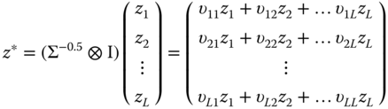
the elements of the matrix ![]() , each variable
, each variable ![]() of the model is transformed by pre‐multiplying it by:
of the model is transformed by pre‐multiplying it by: ![]() . We then have:
. We then have:
The three‐stage least squares estimator is obtained by using the moment conditions: ![]() , for which the variance is:
, for which the variance is: ![]() . Consistently with the method of moments approach, the estimator is obtained by minimizing a quadratic form of the vector of moments, using the inverse of the variance matrix of these moments:
. Consistently with the method of moments approach, the estimator is obtained by minimizing a quadratic form of the vector of moments, using the inverse of the variance matrix of these moments:
First order conditions for a minimum are:
Solving this linear system of equations, we obtain the 3SLS estimator:
The 3SLS estimator may be obtained by employing the instrumental variables estimator, pre‐multiplying the covariates and the response by ![]() and the instruments by
and the instruments by ![]() . The instruments are then
. The instruments are then ![]() and define the following projection matrix:
and define the following projection matrix:
But:
We then have
Using this projection matrix in the formula of the instrumental variables estimator 6.3 we finally get:

or
which is the formula 6.12 of the 3SLS estimator. Of course, as in the GLS estimator, ![]() is in practice unknown and shall be estimated based on the results from a consistent preliminary estimation.
is in practice unknown and shall be estimated based on the results from a consistent preliminary estimation.
The practical computation of the 3SLS estimator consists then of the following steps:
- each equation is first estimated independently using the instrumental variables estimator, which leads to a matrix of residuals
 which is a consistent estimate of the errors of the equations,
 - the covariance matrix of the errors of the system is then estimated:

- the Cholesky decomposition of this matrix is computed:
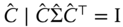 ,
, - the variables are transformed using this matrix:
 ,
,  and
and  .
. - and finally the instrumental variables estimator is applied to the transformed system.
The computation of the within or between 3SLS estimators is straightforward, as it consists in applying the 3SLS to within or between transformed data.
6.4.2 The Error Components Three Stage Least Squares Estimator
Balestra and Varadharajan‐Krishnakumar (1987) and Baltagi (1981) have proposed 3SLS estimators that use the inter‐ and intra‐individual variations of the data in an optimal way.
From now, three indexes must be considered, the individual ![]() and time indexes
and time indexes ![]() as usual, but also the equation index
as usual, but also the equation index ![]() .
.
Denoting by ![]() , the error vector for individual
, the error vector for individual ![]() and equation
and equation ![]() , the error vector for the system of equations is:
, the error vector for the system of equations is:
The covariance matrix of the errors is then:
The presence of individual effects makes this model specific compared to the standard 3SLS estimator. Compared to the standard error component model, scalars ![]() and
and ![]() are replaced by two covariance matrices
are replaced by two covariance matrices ![]() and
and ![]() .
.
The 3SLS estimator can then be computed the following way:
- firstly, the different equations are estimated using 2SLS so that a consistent estimator of the matrix of the errors of the different equations
 may be computed;
 - then,
 and
and  are estimated by
  and
and  ,
, - covariates and responses are transformed by pre‐multiplying them by:
 ,
, - instrumental variables are transformed by pre‐multiplying them by:
 ,
, - the 2SLS estimator is then applied to the transformed data.
As for the 2SLS estimator, the difference between the estimators of Baltagi (1981) and Balestra and Varadharajan‐Krishnakumar (1987) is that the former uses the within and the between transformations of the instruments, while the latter uses a quasi‐difference transformation.
6.5 More Empirical Examples
Acconcia et al. (2014) seek to estimate the multiplier effect of public spending. This is a difficult task, as public spending can hardly be considered exogenous. They use a panel of 95 Italian administrative regions (provinces) for the years 1990‐1999 and take advantage of the implementation of anti‐mafia laws, which resulted in the eviction of some elected officials who were replaced by external commissioners. This replacement, which led to a drastic reduction in local public spending, represents an exogenous source of variation in public spending that can be usefully employed as instrument. Using a fixed effects 2SLS estimator, they estimate the long‐term public spending multiplier to be 1.95, a much larger value than the one obtained using the within estimator. The Mafia dataset is available in the pder package.
Egger and Pfaffermayr (2004) studied the determinants of bilateral trade of two countries, Germany and the United States, with their partners, bilateral trade being measured by imports and exports on the one hand, and by foreign direct investment on the other. The authors suspect that the individual effect, which indicates a propensity to trade with a given country for geographical and cultural reasons, is correlated with the distance. In this case, this variable, which is the only time‐invariant one, is certainly correlated with the individual effect. The authors use the estimator of Hausman and Taylor (1981) for each equation and also for the system of two equations. The data are provided as TradeFDI in the pder package.
Hutchison and Noy (2005) study the effects of twin crises, characterized by the simultaneous occurrence of a bank and a currency crisis, on the wealth of countries. The panel consists of 24 developing countries for the 1975‐1997 period. The response is the growth rate of the GDP and the two main covariates are the lag of the growth rate and a dummy variable indicating the occurrence of a twin crisis. Employing the lag of the growth rate as a covariate induces an endogeneity problem, which the authors tackle using an error component 2SLS estimator. The results indicate that the cost of a currency crisis is about 5‐8% in terms of growth every year for about 2‐4 years, while for the bank crisis this is about 8‐10%. The article doesn't provide any evidence of a specific effect of twin crises. The data are provided as TwinCrises in the pder package.
Cornwell and Trumbull (1994) and Baltagi (2006) estimate a crime economics model for the counties of North Carolina. The response is the criminality rate and, among the covariates, they introduce the probability of being arrested and the number of policemen per inhabitant. These two covariates induce an endogeneity problem: one actually wants to estimate the causal effect of police on crime, but a reverse causality effect is also likely, because more crime will induce the presence of more policemen. Two instrumental variables are used: the offense mix, which is defined as the ratio of crimes involving face‐to‐face contact to those that do not, and the per capita tax revenue. The first instrument is positively correlated with the probability of being arrested (because the offender may be identified by the victim). The second variable is positively correlated with the number of policemen, more tax income indicating a strong preference for public services and particularly for security. The 2SLS error component model indicates a much stronger effect of the probability of being arrested than for the other estimators, especially the within estimator. The data are provided as Crime in the plm package.
Baltagi and Khanti‐Akom (1990) and Cornwell and Rupert (1988) estimate a wage function using a panel of American individuals, with particular interest in the return to education. A well‐known problem of such studies is that unobserved characteristics of individuals, called abilities, are part of the individual effects and may be correlated with education. Using the within model, the education covariate disappears: the use of the estimator of Hausman and Taylor (1981) is therefore very relevant in this context. Two time‐invariant covariates (being black and being a female) are assumed exogenous, while the level of education is endogenous. Some other time‐varying covariates are assumed exogenous and therefore provide two instruments so that the model is identified. The coefficient of education from the Hausman and Taylor (1981) estimator is larger than the one obtained using GLS (0.14 vs 0.10). The data are provided as Wages in the plm package.