

9 Systems of Equations and Inequalities
Chapter Outline
9.1 Systems of Linear Equations
9.2 Determinants and Cramer’s Rule
9.3 Systems of Nonlinear Equations
Introduction Recall from Section 2.3 that a linear equation in two variables x and y is any equation that can be put in the form ax + by = c, where a and b are real numbers and not both zero. In general, a linear equation in n variables x1, x2, …., xn is an equation of the form
![]()
where the real numbers a1, a2, …., an are not all zero. The number b is called the constant term of the equation. The equation in (1) is also called a first-degree equation in that the exponent of each of the n variables is 1. In this and the next section we examine solution methods for systems of equations.
![]() Terminology A system of equations consists of two or more equations with each equation containing at least one variable. If each equation in a system is linear, we say that it is a system of linear equations or simply a linear system. Whenever possible, we will use the familiar symbols x, y, and z to represent variables in a system. For example,
Terminology A system of equations consists of two or more equations with each equation containing at least one variable. If each equation in a system is linear, we say that it is a system of linear equations or simply a linear system. Whenever possible, we will use the familiar symbols x, y, and z to represent variables in a system. For example,

is a linear system of three equations in three variables. The brace in (2) is just a way of reminding us that we are trying to solve a system of equations and that the equations must be dealt with simultaneously. A solution of a system of n equations in n variables consists of values of the variables that satisfy each equation in the system. A solution of such a system is also written as an ordered n-tuple. For example, as we see x = 2, y = −1, and z = 3 satisfy each equation in the linear system (2):

and so these values constitute a solution. Alternatively, this solution can be written as the ordered triple (2, −1, 3). To solve a system of equations we find all solutions of the system. Often to solve a system of equations we perform operations on the system to transform it into an equivalent set of equations. Two systems of equations are said to be equivalent if they have precisely the same solution sets.
![]() Linear Systems in Two Variables The simplest linear system consists of two equations in two variables:
Linear Systems in Two Variables The simplest linear system consists of two equations in two variables:
![]()
Because the graph of a linear equation ax + by = c is a straight line, the system determines two straight lines in the xy-plane.
![]() Consistent and Inconsistent Systems As shown in FIGURE 9.1.1 there are three possible cases for the graphs of the equations in system (3):
Consistent and Inconsistent Systems As shown in FIGURE 9.1.1 there are three possible cases for the graphs of the equations in system (3):
• The lines intersect in a single point. ←Figure 9.1.1(a)
• The equations describe coincident lines. ← Figure 9.1.1(b)
• The two lines are parallel. ← Figure 9.1.1(c)

FIGURE 9.1.1 Two lines in the plane
In these three cases we say, respectively:
- The system is consistent and the equations are independent. The system has exactly one solution, that is, the ordered pair of real numbers corresponding to the point of intersection of the lines.
- The system is consistent, but the equations are dependent. The system has infinitely many solutions, that is, all the ordered pairs of real numbers corresponding to the points on the one line.
- The system is inconsistent. The lines are parallel and so there are no solutions.
For example, the equations in the linear system
![]()
are parallel lines as in Figure 9.1.1(c). Hence the system is inconsistent.
To solve a system of linear equations, we can use either the method of substitution or the method of elimination.
![]() Method of Substitution The first solution technique considered is called the method of substitution.
Method of Substitution The first solution technique considered is called the method of substitution.
EXAMPLE 1 Method of Substitution
Solve the linear system
![]()
Solution Solving the second equation for y yields
y = 2x − 4.
We substitute this expression into the first equation and solve for x:
3x + 4(2x − 4) = −5 or 11x = 11 x = 1.
We then substitute this value back into the first equation:
![]()
![]() Back-substitution
Back-substitution
Thus the only solution of the system is (1, −2). The system is consistent and the equations are independent.
![]() Solution written as an ordered pair.
Solution written as an ordered pair.
![]() Linear Systems in Three Variables In Section 7.5 we saw that the graph of a linear equation in three variables,
Linear Systems in Three Variables In Section 7.5 we saw that the graph of a linear equation in three variables,
ax + by + cz = d,
where a, b, and c are not all zero, is a plane in three-dimensional space. As we have seen in (2), a solution of a system of three equations in three variables

is an ordered triple of the form (x, y, z); an ordered triple of numbers represents a point in three-dimensional space. The intersection of the three planes described by the system (4) may be
• a single point,
• infinitely many points, or
• no points.
As before, to each of these cases we apply the terms consistent and independent, consistent and dependent, and inconsistent, respectively. Each is illustrated in FIGURE 9.1.2.

FIGURE 9.1.2 Three planes in three dimensions
![]() Method of Elimination The next method that we illustrate uses elimination operations. When applied to a system of equations, these operations yield an equivalent system of equations.
Method of Elimination The next method that we illustrate uses elimination operations. When applied to a system of equations, these operations yield an equivalent system of equations.
We often add a nonzero constant multiple of one equation to other equations in a system with the intention of eliminating a variable from those equations.
For convenience, we represent these operations by the following symbols, where the letter E stands for the word equation:
Ei ↔ Ej: Interchange the ith equation with the jth equation.
kEi: Multiply the ith equation by a constant k.
kEi + Ej: Multiply the ith equation by k and add to the jth equation.
Reading a linear system from the top, E1 represents the first equation, E2 represents the second equation, and so on.
Using the method of elimination it is possible to reduce the system (4) of three linear equations in three variables to an equivalent system in triangular form,

A solution of the system (if one exists) can be readily obtained by back-substitution. The next example illustrates the procedure.
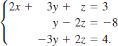
EXAMPLE 2 Elimination and Back-Substitution
Solve the linear system

Solution We begin by eliminating x from the second and third equations:
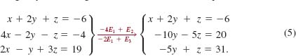
We then eliminate y from the third equation and obtain an equivalent system in triangular form:

We arrive at another triangular form that is equivalent to the original system by multiplying the third equation by ![]()

From this last system it is evident that z = 6. Using this value and substituting back into the second equation gives
![]()
Finally, by substituting y = −5 and z = 6 back into the first equation, we obtain
x = −2y − z −6 = −2(−5) −6 −6 = −2.
Therefore the solution of the system is (−2, −5, 6).
![]() The answer indicates that the three planes intersect at a point as in Figure 9.1.2 (a).
The answer indicates that the three planes intersect at a point as in Figure 9.1.2 (a).
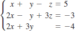
EXAMPLE 3 Elimination and Back-Substitution
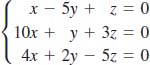
Solve the linear system

Solution Using the first equation to eliminate the variable x from the second and third equations, we get the equivalent system
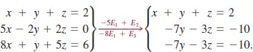
This system, in turn, is equivalent to the system in triangular form:

In this system we cannot determine unique values for x, y, and z. At best we can solve for two variables in terms of the remaining variable. For example, from the second equation in (8), we obtain y in terms of z:
![]()
Substituting this equation for y in the first equation for x gives
![]()
Thus in the solutions for y and x, we can choose z arbitrarily. If we denote z by the symbol where represents a real number, then the solutions of the system are all ordered triples of the form ![]() We emphasize that for any real number we obtain a solution of (7). For example, by choosing to be, say, 0, 1, and 2, we obtain the solutions
We emphasize that for any real number we obtain a solution of (7). For example, by choosing to be, say, 0, 1, and 2, we obtain the solutions ![]() respectively. In other words, the system is consistent and has infinitely many solutions.
respectively. In other words, the system is consistent and has infinitely many solutions.
![]() The answer indicates that the two planes intersect in a line as in Figure 9.1.2 (b).
The answer indicates that the two planes intersect in a line as in Figure 9.1.2 (b).
In Example 3 there is nothing special about solving (8) for x and y in terms of z. For instance, by solving (8) for x and z in terms of y, we obtain the solution ![]() where is any real number. Note that by setting β equal to 10/7, 1, and we get the same solutions in Example 3 corresponding, in turn, to and α = 0, α = 1, and α = 2.
where is any real number. Note that by setting β equal to 10/7, 1, and we get the same solutions in Example 3 corresponding, in turn, to and α = 0, α = 1, and α = 2.
EXAMPLE 4 No Solution
Solve the linear system

Solution The elimination method,

shows that the last equation 0z = 3 is never satisfied for any number z since 0 ≠ 3. Thus, the system is inconsistent and so has no solutions.

FIGURE 9.1.3 Inclined plane in Example 5
EXAMPLE 5 Elimination and Back-Substitution
A force of smallest magnitude P is applied to a 300-lb block on an inclined plane in order to keep it from sliding down the plane. See FIGURE 9.1.3. If the coefficient of friction between the block and the surface is 0.4, then the magnitude of the frictional force is 0.4N, where N is the magnitude of the normal force exerted on the block by the plane. Since the system is in equilibrium, the horizontal and the vertical components of the forces must be zero:
![]()
Solve this system for P and N.
Solution Using ![]() we simplify the system above to
we simplify the system above to

By elimination,

The second equation of the last system gives N = 150![]() ≈ 259.81 lb. By substituting this value into the first equation we obtain P = 150(1 − 0.4
≈ 259.81 lb. By substituting this value into the first equation we obtain P = 150(1 − 0.4![]() ) ≈ 46.08lb.
) ≈ 46.08lb.
![]() Homogeneous Systems A linear system in which all the constant terms are zero, such as
Homogeneous Systems A linear system in which all the constant terms are zero, such as
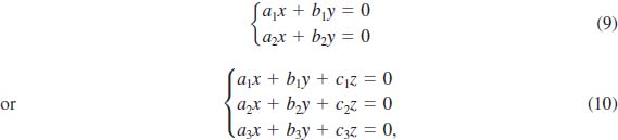
is said to be homogeneous. Note that systems (9) and (10) have the solutions (0, 0) and (0, 0, 0), respectively. A solution of a system of equations in which each of its variables is zero is called the zero solution or the trivial solution. Because a homogeneous linear system always possesses at least the zero solution, such a system is always consistent. In addition to the zero solution, however, there may exist infinitely many nonzero solutions. These solutions can be found by proceeding exactly as in Example 3.
![]() A homogeneous system is consistent even in the case where the linear system consists of m equations in n variables, where m ≠ n.
A homogeneous system is consistent even in the case where the linear system consists of m equations in n variables, where m ≠ n.
EXAMPLE 6 A Homogeneous System
The same steps used to solve the system in Example 3 can be used to solve the related homogeneous system

In this case the elimination steps yield

Choosing z = α, where α is a real number, we find from the second equation of the last system that ![]() Then using the first equation, we obtain
Then using the first equation, we obtain ![]() Thus, the solutions of the system consist of all ordered triples of the form
Thus, the solutions of the system consist of all ordered triples of the form ![]() Note that for α = 0, we obtain the trivial solution (0, 0, 0) but for, say, α = −7, we obtain the nontrivial solution (4, 3, −7).
Note that for α = 0, we obtain the trivial solution (0, 0, 0) but for, say, α = −7, we obtain the nontrivial solution (4, 3, −7).
The two techniques in this section are also applicable to systems of n linear equations in n variables for n > 3. See Problems 25 and 26 in Exercises 9.1. In addition, these techniques are applicable to linear systems where the number of equations is not the same as the number of variables. See Problems 27–30 in Exercises 9.1. In the following example, we consider a system of 2 equations in 3 variables.
![]() Note
Note
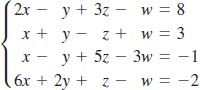
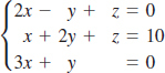
EXAMPLE 7 Two Equations in Three Variables
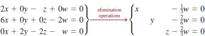
Use method of elimination to solve the linear system
![]()
Solution We have

The last system indicates that x = 0 and y = 2z + 3. As in Examples 3 and 6, we may now assign any value to z. Hence the solutions of the system are all ordered triples of the form (0, 2α + 3, α) where is any real number.
A homogeneous linear system, regardless of the number equations and variables is consistent. In our last example we consider an example from chemistry where we must solve a homogeneous system of 3 equations in 4 variables.
EXAMPLE 8 Balancing a Chemical Equation
Balance the chemical equation C2H6 + O2 → CO2 + H2O.
Solution We seek positive integers x, y, z and w so that the balanced equation is
xC2H2 + yO2 → zCO2 + wH2O.
Because the number of atoms of each element must be the same on each side of the last equation, we obtain the homogeneous system of 3 equations in 4 variables:

Since the last system is homogeneous it must be consistent. Using elementary row operations, we find
and so a solution of the system is ![]() In this case α must be a positive integer chosen in such a manner so that x, y, z and w are positive integers. To accomplish this we pick α = 6. This gives x = 2, y = 7, z = 4, and w = 6. The balanced equation is then
In this case α must be a positive integer chosen in such a manner so that x, y, z and w are positive integers. To accomplish this we pick α = 6. This gives x = 2, y = 7, z = 4, and w = 6. The balanced equation is then
2C2H6 + 7O2 → 4CO2 + 6H2O.
9.1 Exercises Answers to selected odd-numbered problems begin on page ANS-26.
In Problems 1–26, solve the given linear system. State whether the system is consistent, with independent or dependent equations, or whether it is inconsistent.
1. ![]()
2. ![]()
3. ![]()
4. ![]()
5. ![]()
6. ![]()
7. ![]()
8. ![]()
9. ![]()
10. ![]()
11. 
12. 
13. 
14. 
15. 
16. 
17. 
18. 
19. 
20. 
21. 
22. 
23. 
24. 
25. 
26. 
In Problems 27–30, solve the given linear system.
27. ![]()
28. ![]()
29. 
30. ![]()
In Problems 31–36, use the procedure illustrated in Example 8 to balance the given chemical equation.
31. Na + H2O → NaOH + H2
32. KCIO3 → KCI + O2
33. Fe3O4 + C → Fe + CO
34. C5H8 + O2 → CO2 + H2O
35. Cu + HNO3 → Cu(NO3)2 + H2O + NO
36. Ca3(PO4)2 + H3PO4 → Ca(H2PO4)2
In Problems 37–40, each system is nonlinear in the given variables. Use substitutions to convert the system into one that is linear in the new variables. Solve, and then give the solution of the original system.
37. 
38. 
39. ![]()
40. ![]()
41. The magnitudes T1 and T2 of the tensions in the two cables shown in FIGURE 9.1.4 satisfy the system of equations
![]()
Find T1 and T2.
42. If we change the direction of the frictional force in Figure 9.1.3 of Example 5, then the system of equations becomes

In this case, P represents the magnitude of the force that is just enough to start the block up the plane. Find P and N.

FIGURE 9.1.4 Cables in Problem 41
Miscellaneous Applications
43. Speed An airplane flies 3300 mi from Hawaii to California in 5.5 h with a tailwind. From California to Hawaii, flying against a wind of the same velocity, the trip takes 6 h. Determine the speed of the plane and the speed of the wind.
44. How Many Coins? A person has 20 coins, consisting of dimes and quarters, which total $4.25. Determine how many of each coin the person has.
45. Number of Gallons A 100-gal tank is full of water in which 50 lb of salt is dissolved. A second tank contains 200 gal of water with 75 lb of salt. How much should be removed from both tanks and mixed together in order to make a solution of 90 gal with of ![]() lb salt per gallon?
lb salt per gallon?
46. Playing with Numbers The sum of three numbers is 20. The difference of the first two numbers is 5, and the third number is 4 times the sum of the first two. Find the numbers.
47. How Long? Three pumps P1, P2, and P3 working together can fill a tank in 2 hours. Pumps P1 and P2 can fill the same tank in 3 hours, whereas pumps P2 and P3 can fill it in 4 hours. Determine how long it would take each pump working alone to fill the tank.
48. Parabola Through Three Points The parabola y = ax2 + bx + c passes through the points (1, 10), (−1, 12), and (2, 18). Find a, b, and c.
49. Area Find the area of the right triangle shown in FIGURE 9.1.5.

FIGURE 9.1.5 Triangle in Problem 49
50. Current According to Kirchhoff’s law of voltages, the currents i1, i2, and i3 in the parallel circuit shown in FIGURE 9.1.6 satisfy the equations

Solve for i1, i2, and i3.

FIGURE 9.1.6 Circuit in Problem 50
51. The A, B, C’s When Beth graduated from college, she had completed 40 courses, in which she received grades of A, B, and C. Her final GPA (grade point average) was 3.125. Her GPA in only those courses in which she received grades of A and B was 3.8. Assume that A, B, and C grades are worth four points, three points, and two points, respectively. Determine the number of A’s, B’s, and C’s that Beth received.
52. Conductivity Cosmic rays are deflected toward the poles by the Earth’s magnetic field, so that only the most energetic rays can penetrate the equatorial regions. See FIGURE 9.1.7. As a result, the ionization rate, and hence the conductivity σ of the stratosphere, is greater near the poles than it is near the equator. Conductivity can be approximated by the formula
![]()
where φ is latitude and A and B are constants that must be chosen to fit the physical data. Balloon measurements made in the southern hemisphere indicated a conductivity of approximately 3.8 × 10⁻¹² siemens/meter at 35.5° south latitude and 5.6 × 10⁻¹² siemens/meter at 51° south latitude. (A siemen is the reciprocal of an ohm, which is a unit of electrical resistance.) Determine the constants A and B. What is the conductivity at 42° south latitude?

FIGURE 9.1.7 Earth’s magnetic field in Problem 52
For Discussion
53. Determine conditions on a1, a2, b1, and b2 so that the linear system (9) has only the trivial solution.
54. Determine a value of k such that the linear system
![]()
is (a) inconsistent, and (b) dependent.
55. Devise a system of two linear equations whose solution is (2, −5).
Introduction If a linear system of equations has the same number of equations as it does variables, say two equations and two variables, then it may be possible to solve the system using determinants. If a11, a12, … represent real numbers, then the symbols
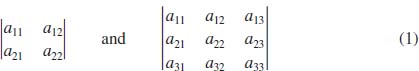
are called determinants of order 2 and order 3, respectively. Although a determinant can be any order n, n a positive integer, most of the elementary applications of determinants in calculus utilize second- and third-order determinants.
![]() Determinant of Order 2 A determinant is a number. In the case of a determinant of order 2 we have the following definition.
Determinant of Order 2 A determinant is a number. In the case of a determinant of order 2 we have the following definition.
DEFINITION 9.2.1 Determinant of Order 2
A determinant of order 2 is the number
![]()
EXAMPLE 1 Determinant of Order 2
Evaluate the determinant ![]()
Solution From (2) of Definition 9.2.1,
![]()
As a mnemonic for the formula in (2), remember that the determinant is the difference of the products of the diagonal entries:

Even though a determinant is a number it is convenient to think of it as a square array. Thus determinants of orders 2 and 3 are also referred to as 2 × 2 (read “two by two”) and 3 × 3 (“three by three”) determinants, respectively.
Determinants of order 2 play a fundamental role in the evaluating of determinants of order n, n > 2. In general, a determinant of order n can be expressed in terms of determinants of order n – 1. Thus, for example, a 3 × 3 determinant can be expressed in terms of determinants of order 2. In preparation for a method for finding the value of a 3 × 3 determinant we need to introduce the notion of a cofactor determinant.
![]() Minor and Cofactor If aij denotes the entry in the ith row and jth column of a determinant of order n, then the minor Mij of aij is defined to be the determinant of order n – 1 obtained by deleting the row and the column of the determinant of order n. Thus for 3 × 3 the determinant
Minor and Cofactor If aij denotes the entry in the ith row and jth column of a determinant of order n, then the minor Mij of aij is defined to be the determinant of order n – 1 obtained by deleting the row and the column of the determinant of order n. Thus for 3 × 3 the determinant

the minors of a11 = 1,a12 = 5,a22 = 4, and a32 = 2 are, in turn, the determinants

The cofactor Aij of the entry aij is defined to be the minor Mij multiplied by (−1)i+j that is,
![]()
![]() (−1)i+j is 1 if i + j is even, (−1)i+j is −1 if i + j is odd.
(−1)i+j is 1 if i + j is even, (−1)i+j is −1 if i + j is odd.
Thus for the determinant in (3) the cofactors associated with the foregoing minor determinants are

and so on. For a 3 × 3 determinant, the coefficient (−1)i+j of the minor Mij follows the pattern

This “checkerboard” pattern of signs extends to determinants of greater order as well.
EXAMPLE 2 Cofactors
Find the cofactor of the given entry: (a) 0 (b) (c) −1 for the determinant

Solution (a) The number 0 is the entry of the first row (i = 1) and third column (j = 3). From (4) the cofactor of 0 is the determinant
![]()
(b) The number 7 is the entry in the second row (i = 2) and third column (j = 3). Thus the cofactor is
![]()
(c) Finally, because −1 is the entry in the third row (i = 3)and first column (j = 1), its cofactor is
![]()
We are now in a position to find the value of a determinant of order 3. Although the next theorem is stated for 3 × 3 determinants, it is equally valid for any determinant of order n.
THEOREM 9.2.1 Expansion Theorem
The value of a 3 × 3 determinant can be found by multiplying each entry in any row (or column) by its cofactor and adding the results.
When we use Theorem 9.2.1 to find the value of a determinant we say that we have expanded the determinant of A by a given row or by a given column. For example, the expansion of the determinant of the 3 × 3 matrix in (1) by the first row is

EXAMPLE 3 Expansion by the First Row
Evaluate the 3 × 3 determinant

Solution Using the expansion by the first row given in (5) we have

Theorem 9.2.1 states that a determinant can be expanded by any row or any column. For example, the expansion of the 3 × 3 determinant in (1) by, say, the second row is

EXAMPLE 4 Example 3 Revisited
The expansion of the determinant in Example 3 by the third column is

In the expansion of a determinant, since the entries in a row (or column) multiply the cofactors of that row (or column), it makes sense that if a determinant has a row (or column) with several 0 entries that we expand the determinant by that row (or column). It also follows, that if a determinant has an entire row (or column) of 0 entries, then the value of the determinant is 0.
![]() Note
Note
![]() Cramer’s Rule Suppose the linear equations
Cramer’s Rule Suppose the linear equations
![]()
are independent. If we multiply the first equation by b2 and the second by −b1 we obtain the equivalent system
![]()
Then we can eliminate the y-variable and solve for x by adding the two equations:

Similarly, by eliminating the x-variable, we find
![]()
The numerators and the common denominator in (7) and (8) can be written as 2 × 2 determinants. If we denote these determinants by
![]()
then we can summarize the discussion in a compact fashion.
THEOREM 9.2.2 Two Equations in Two Variables
If D ≠ 0, then the system (6) has the unique solution
![]()
By comparing the determinant D in (9) with the system (6) we see that D is the determinant of the coefficients of x and y. Moreover, a careful inspection of Dx and Dy reveals that these determinants are, in turn, D with the x-coefficients and the y-coefficients replaced by the numbers c1 and c2.
EXAMPLE 5 Using (10)
Solve the linear system
![]()
Solution Since
![]()
Theorem 9.2.2 guarantees that the system has a unique solution. Continuing, we find
![]()
From (10) the solution is given by
![]()
In like manner, the solution (10) can be extended to larger systems of linear equations. In particular, for a system of three equations in three variables,
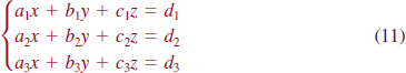
the determinants that correspond to those in (9) are

As in (10), the determinants Dx, Dy, and Dz are obtained from the determinant D of the coefficients of the system, by replacing the x-, y-, and z-coefficients, respectively, by the numbers d1, d2 and d3. The solution of (11) that is analogous to (10) is given next.
THEOREM 9.2.3 Three Equations in Three Variables
If D ≠ 0, then the system (11) has the unique solution
![]()
The solutions in (10) and (13) are special cases of a more general method known as Cramer’s Rule, named after the Swiss mathematician Gabriel Cramer (1704–1752) who was the first to publish these results.
EXAMPLE 6 Using Cramer’s Rule
Solve the linear system

Solution We must evaluate four determinants using the cofactor expansion (4). We begin by finding the value of the determinant of the coefficients of the variables in the system:

The fact that this determinant is nonzero is sufficient to indicate that the system is consistent and has a unique solution. Continuing, we find
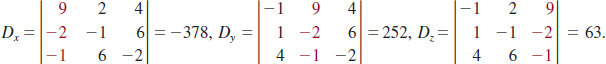
From (13), the solution of the system is then
![]()
EXAMPLE 7 Using Cramer’s Rule
Solve the linear system
Solution As in Example 6 we begin by finding the value of the determinant of the coefficients of the variables:

Because the first column of this determinant has two zero entries we expand D by the first column:
![]()
Because D ≠ 0 we continue and find the values

From (13), the solution of the system is then
![]()
When the determinant D of the coefficients of the variables in a linear system is 0, Cramer’s Rule cannot be used. As we see in the next example, this does not mean the system has no solution.
EXAMPLE 8 Consistent System
For the linear system
![]()
we see that
![]()
Although we cannot apply (10), the method of elimination would show us that the system is consistent but that the equations in the system are dependent.
As mentioned previously, Cramer’s Rule can be extended to systems of n linear equations in n variables for n > 3. But as a practical matter, Cramer’s Rule is seldom used on systems with a large number of equations simply because evaluating the determinants by hand becomes a Herculean task.
9.2 Exercises Answers to selected odd-numbered problems begin on page ANS–26.
In Problems 1–4, find the minor and cofactor determinants for each entry in the given determinant.
1. ![]()
2. ![]()
3. 
4. 
In Problems 5–18, evaluate the given determinant. In Problem 10, assume that a ≠ 0, b ≠ 0.
5. ![]()
6. ![]()
7. ![]()
8. ![]()
9. ![]()
10. ![]()
11. 
12. 
13. 
14. 
15. 
16. 
17. 
18. 
In Problems 19–34, use Cramer’s Rule, if applicable, to solve the given linear system.
19. ![]()
20. ![]()
21. ![]()
22. ![]()
23. ![]()
24. ![]()
25. ![]()
26. ![]()
27. 
28. 
29. 
30. 
31. 
32. 
33. 
34. 
In Problems 35 and 36, solve for x.
35. 
36. 
In Problems 37–40, verify the given identity by evaluating each determinant.
37. ![]()
38. ![]()
39. ![]()
40. ![]()
41. Show that

42. Verify that an equation of the line through the points (x1, y1), (x2, y2) is given by

In Problems 43–46, find the values of λ for which given determinant is 0.
43. ![]()
44. ![]()
45. 
46. 

FIGURE 9.2.1 Echo sounding procedure in Problem 47
Miscellaneous Applications
47. Echo Sounding This problem shows how the depth of an ocean and the speed of sound in water can be measured by a procedure known as echo sounding. Suppose that an oceanographic vessel emits sonar signals and that the arrival times of the signals reflected from the flat ocean floor are recorded at two trailing sonobuoys. See FIGURE 9.2.1. Using the relation distance = rate × time, we see from the figure that 2l2 = vt1 and 2l2 = vt2, where is the speed of sound in water, t1 and t2 are the arrival times of the signals at the two sonobuoys, and l1 and l2 are the indicated distances.
(a) Show that the speed of sound in water v and ocean depth D satisfy the system of equations
![]()
[Hint: Use the Pythagorean theorem to relate l1, d1, and D, and l2, l2 and D.]
(b) Use Cramer’s Rule to solve the system of equations in part (a) to obtain formulas for v2 and D2. Then express v and D in terms of the measurable quantities d1, d2, t1, and t2.
(c) The sonobuoys, trailing at 1000 m and 2000 m, record the arrival times of the reflected signals at 1.4 s and 1.8 s, respectively. Find the depth of the ocean and the speed of sound in water.
48. Take Your Vitamins The United States recommended daily allowance (U.S. RDA), in percent of vitamin content per ounce of food groups X, Y, and Z, is given in the following table.
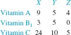
Use Cramer’s Rule to determine how many ounces of each food group one must consume each day in order to get 100% of the daily recommended allowance of vitamin A. 30% of the daily recommended allowance of vitamin B1, and 200% of the daily recommended allowance of vitamin C.
For Discussion
In Problems 49 and 50, evaluate each determinant given that

49. 
50. 
In Problems 51 and 52, extend Theorem 9.2.1 to 4 × 4 determinants and then evaluate the given determinant.
51. 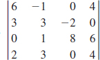
52. 

FIGURE 9.3.1 Intersection of two parabolas
Introduction As FIGURE 9.3.1 illustrates, the graphs of the parabolas y = x2 − 4x and y = −x2 + 8 intersect at two points. Thus the coordinates of the points of intersection must satisfy both equations,
![]()
Recall from Sections 2.3 and 9.1 that any equation that can be put in the form ax + by + c = 0 is called a linear equation in two variables. A nonlinear equation is simply one that is not linear. For example, in system (1) both equations y = x2 − 4x and y = −x2 + 8 are nonlinear. A system of equations in which at least one of the equations is nonlinear will be referred to as a system of nonlinear equations or simply a nonlinear system.
In the examples that follow, will use the methods of substitution and elimination introduced in Section 9.1 to solve nonlinear systems.
EXAMPLE 1 Solution of (1)
Find solutions of system (1).
Solution Since the first equation already expresses y in terms of x, we substitute this expression for y into the second equation to get a single equation in one variable:
x2 − 4x = −x2 + 8.
Simplifying the last equation we get a quadratic equation x2 − 2x − 4 = 0 that we solve using the quadratic formula: x = 1 − ![]() and x = 1 +
and x = 1 + ![]() We then substitute each of these numbers back into the first equation in (1) to solve for the corresponding values of y. This gives
We then substitute each of these numbers back into the first equation in (1) to solve for the corresponding values of y. This gives
![]()
Thus, (1 − ![]() + 2
+ 2![]() ) and (1 +
) and (1 + ![]() , 2 − 2
, 2 − 2![]() are solutions of the system.
are solutions of the system.
EXAMPLE 2 Solving a Nonlinear System
Find solutions of the nonlinear system
![]()
Solution From the second equation, we have x = 10y, and therefore x2 = 102y. Substituting this last result into the first equation gives
![]()
Since x2 + 1 > 0 for all real numbers x, it follows that ![]() But x = 10y > 0 for all y; therefore, we must take x =
But x = 10y > 0 for all y; therefore, we must take x = ![]() Solving
Solving ![]() = 10y for y gives
= 10y for y gives
![]()
Hence, ![]() is the only real solution of the system.
is the only real solution of the system.
![]() Solution written by specifying values of the variables.
Solution written by specifying values of the variables.
Nonlinear systems of equations can have complex solutions. Observe in Example 2 that equation (2) is also satisfied when x2 + 1 = 0 or for x = ≠i, where ![]() The corresponding values of y are also complex but will not be given since that entails working with the logarithm of a complex number. For the rest of this section we are concerned only with finding the real solutions of nonlinear systems.
The corresponding values of y are also complex but will not be given since that entails working with the logarithm of a complex number. For the rest of this section we are concerned only with finding the real solutions of nonlinear systems.
EXAMPLE 3 Dimensions of a Rectangle
Consider a rectangle in the first quadrant bounded by the x- and y-axes and the graph of y = 20 − x2. See FIGURE 9.3.2. Find the dimensions of such a rectangle if its area is 16 square units.

FIGURE 9.3.2 Rectangle in Example 3
Solution Let (x, y) be the coordinates of the point P on the graph of y = 20 − x2 shown in the figure. Then the
area of the rectangle = xy 16 = xy
Thus we obtain the system of equations
![]()
The first equation of the system yields y = 16/x.After substituting this expression for y in the second equation, we get

Now from the Rational Zeros Theorem in Section 3.4 the only possible rational roots of the last equation are ±1, ±2, ±4, ±8, and ±16. Testing these numbers by synthetic division eventually shows that

and so 4 is a solution. But the division above gives the factorization
x3 − 20x + 16 = (x − 4)(x2 + 4x − 4).
Applying the quadratic formula to x2 + 4x − 4 = 0 reveals two more real roots:
![]()
The positive number −2 + 2![]() is another solution. Since dimensions are positive, we reject the negative number −2 + 2
is another solution. Since dimensions are positive, we reject the negative number −2 + 2![]() In other words, there are two rectangles with area 16 square units.
In other words, there are two rectangles with area 16 square units.
To find y, we use y = 16/x. If x = 4, then y = 4, and if ![]() , then
, then ![]() Thus the dimensions of the two rectangles are
Thus the dimensions of the two rectangles are
4 × 4 and 0.83 × 19.31 (approximately).
Note: In Example 3 observe that the equation 16 = 20x − x3 was obtained by multiplying the equation preceding it by x. Remember, when equations are multiplied by a variable, there is the possibility of introducing an extraneous solution. To make sure that this is not the case, you should check each solution.

FIGURE 9.3.3 Intersection of a circle and a hyperbola in Example 4
EXAMPLE 4 Solving a Nonlinear System
Solve the nonlinear system
![]()
Solution In preparation for eliminating an x2-term, we begin by multiplying the first equation by 2. The system
![]()
is equivalent to the given system. Now, by adding the first equation of this last system to the second, we obtain yet another system equivalent to the original system. In this case, we have eliminated x2 from the second equation:
![]()
From the last equation, we see that ![]() Substituting these two values of y into x2 + y2 = 4 then gives
Substituting these two values of y into x2 + y2 = 4 then gives
![]()
so that ![]() are all solutions. The graphs of the given equations and the four points corresponding to the ordered pairs are indicated by the red dots in FIGURE 9.3.3.
are all solutions. The graphs of the given equations and the four points corresponding to the ordered pairs are indicated by the red dots in FIGURE 9.3.3.
In Example 4 we note that the system can also be solved by the substitution method by substituting, say, y2 = 4 − x2 into the second equation.
In the next example, we use the third elimination operation to simplify the system before applying the substitution method.
EXAMPLE 5 Solving a Nonlinear System
Solve the nonlinear system
![]()
Solution By multiplying the first equation by −1 and adding the result to the second, we eliminate x2 and y2 from that equation:
![]()
The second equation of the latter system implies that y = x. Substituting this expression into the first equation then yields
x2 − 2x + x2 = 0 or 2x(x − 1) = 0.
It follows that x = 0, x = 1 and, correspondingly, y = 0, y = 1. Thus solutions of the system are (0, 0) and (1, 1).
By completing the square in x and y, we can write the system in Example 5 as
![]()
From this system we see that both equations describe circles of radius r = 1. The circles and their points of intersection are illustrated in FIGURE 9.3.4.
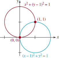
FIGURE 9.3.4 Intersecting circles in Example 5
9.3 Exercises Answers to selected odd-numbered problems begin on page ANS-26.
In Problems 1–6, determine graphically whether the given nonlinear system has any solutions.
1. ![]()
2. ![]()
3. ![]()
4. ![]()
5. ![]()
6. ![]()
In Problems 7–42, solve the given nonlinear system.
7. ![]()
8. ![]()
9. ![]()
10. ![]()
11. ![]()
12. ![]()
13. 
14. ![]()
15. ![]()
16. ![]()
17. ![]()
18. ![]()
19. ![]()
20. ![]()
21. ![]()
22. ![]()
23. ![]()
24. ![]()
25. ![]()
26. ![]()
27. ![]()
28. ![]()
29. ![]()
30. ![]()
31. ![]()
32. ![]()
33. ![]()
34. ![]()
35. ![]()
36. ![]()
37. ![]()
38. ![]()
39. 
40. 
41. 
42. 

FIGURE 9.3.5 Rectangle in Problem 44

FIGURE 9.3.6 Circles in Problem 46
Miscellaneous Applications
43. Dimensions of a Corral The perimeter of a rectangular corral is 260 ft and its area is 4000 ft2. What are its dimensions?
44. Inscribed Rectangle Find the dimensions of the rectangle(s) with area 10 cm2 inscribed in the triangle consisting of the blue line and the two coordinate axes shown in FIGURE 9.3.5.
45. Sum of Areas The sum of the radii of two circles is 8 cm. Find the radii if the sum of the areas of the circles is 32∏ cm2.
46. Intersecting Circles Find the two points of intersection of the circles shown in FIGURE 9.3.6 if the radius of each circle is ![]() .
.
47. Golden Ratio The golden ratio for the rectangle shown in FIGURE 9.3.7 is defined by
![]()
This ratio is often used in architecture and in paintings. Find the dimensions of a rectangular sheet of paper containing 100 in.2 that satisfy the golden ratio.
48. Length The hypotenuse of a right triangle is 20 cm. Find the lengths of the remaining two sides if the shorter side is one-half the length of the longer side.
49. Topless Box A box is to be made with a square base and no top. See FIGURE 9.3.8. The volume of the box is to be 32 ft3, and the combined areas of the sides and bottom are to be 68 ft2. Find the dimensions of the box.
50. Dimensions of a Cylinder The volume of a right circular cylinder is 63π in.3, and its height h is 1 in. greater than twice its radius r. Find the dimensions of the cylinder.

FIGURE 9.3.7 Rectangle in Problem 47

FIGURE 9.3.8 Open box in Problem 49
For Discussion
51. A tangent to an ellipse is defined exactly as it was for the circle, namely, a straight line that touches the ellipse at only one point (x1, y1). See Problem 52 in Exercises 2.3. It can be shown (see Problem 52 that follows) that an equation of the tangent line at a given point (x1, y1) on an ellipse x2⁄a2 + y2⁄b2 = 1 is
![]()
(a) Find the equation of the tangent line to the ellipse x2⁄50 1 y2⁄8 = 1 at the point (5, −2).
(b) Write your answer in the form of y = mx + b.
(c) Sketch the ellipse and the tangent line.
52. In this problem, you are guided through the steps to derive equation (4).
(a) An alternative form of the equation x2⁄a2 + y2⁄b2 = 1 is
b2x2 + a2y2 = a2b2.
Since the point (x1, y1) is on the ellipse, its coordinates must satisfy the foregoing equation:
b2x12 + a2y12 = a2b2.
Show that
b2(x2 − x12) + a2(y2 − y12) = 0.
(b) Using the point-slope form of a line, the tangent line at (x1, y1) is y − y1 = m(x − x1). Use substitution in the system
![]()
to show that
![]()
The last equation is a quadratic equation in x. Explain why x1 is a repeated root or a root of multiplicity 2.
(c) By factoring, (5) becomes
![]()
and so we must have
![]()
Use the last equation to find the slope m of the tangent line at (x1, y1). Finish the problem by finding the equation of the tangent as given in (4).
Introduction In Chapter 1 we solved linear and nonlinear inequalities involving a single variable x and then graphed the solution set of the inequality on the number line. In this section our focus will be on inequalities involving two variables x and y. For example,
![]()
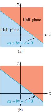
FIGURE 9.4.1 A single line determines two half-planes
are inequalities in two variables. A solution of an inequality in two variables is any ordered pair of real numbers (x0, y0) that satisfies the inequality—that is, results in a true statement—when x0 and y0 are substituted for x and y, respectively. A graph of the solution set of an inequality in two variables is made up of all points in the plane whose coordinates satisfy the inequality.
Many results obtained in calculus are valid only in a specialized region either in the xy-plane or in three-dimensional space, and these regions are often defined by means of systems of inequalities in two or three variables. In this section we consider only systems of inequalities involving two variables x and y.
We begin with linear inequalities in two variables.
![]() Half-Planes A linear inequality in two variables x and y is any inequality that has one of the forms
Half-Planes A linear inequality in two variables x and y is any inequality that has one of the forms
![]()
Since the inequalities in (1) and (2) have infinitely many solutions, the notation
![]()
and so on, is used to denote a set of solutions. Geometrically, each of these sets describes a half-plane. As shown in FIGURE 9.4.1, the graph of the linear equation ax + by + c = 0 divides the xy-plane into two regions, or half-planes. One of these half-planes is the graph of the set of solutions of the linear inequality. If the inequality is strict, as in (1), then we draw the graph of ax + by + c = 0 as a dashed line, because the points on the line are not in the set of solutions of the inequality. See Figure 9.4.1(a). On the other hand, if the inequality is nonstrict, as in (2), the set of solutions includes the points satisfying ax + by + c = 0, and so we draw the graph of the equation as a solid line. See Figure 9.4.1(b).

FIGURE 9.4.2 Half-plane in Example 1
EXAMPLE 1 Graph of a Linear Inequality
Graph the linear inequality 2x − 3y ≥ 12.
Solution First, we graph the line 2x − 3y = 12, as shown in FIGURE 9.4.2(a). Solving the given inequality for y gives
![]()
Since the y-coordinate of any point (x, y) on the graph of 2x − 3y ≥ 12 must satisfy (3), we conclude that the point (x, y) must lie on or below the graph of the line. This solution set is the region that is shaded blue in Figure 9.4.2(b).
Alternatively, we know that the set
![]()
describes a half-plane. Thus we can determine whether the graph of the inequality includes the region above or below the line 2x − 3y = 12 by determining whether a test point not on the line, such as (0, 0), satisfies the original inequality. Substituting x = 0, y = 0 into 2x − 3y ≥ 12 gives 0 ≥ 12. This false statement implies that the graph of the inequality is the region on the other side of the line 2x − 3y = 12, that is, the side that does not contain the origin. Note that the blue half-plane in Figure 9.4.2(b) does not contain the point (0, 0).
In general, given a linear inequality of the forms in (1) or (2), we can graph the solutions by proceeding in the following manner.
- Graph the line ax + by + c = 0.
- Select a test point not on this line.
- Shade the half-plane containing the test point if its coordinates satisfy the original inequality. If they do not satisfy the inequality, shade the other half-plane.
EXAMPLE 2 Graph of a Linear Inequality
Graph the linear inequality 3x + y − 2 < 0.
Solution In FIGURE 9.4.3 we draw the graph of 3x + y = 2 as a dashed line, since it will not be part of the solution set of the inequality. Then we select (0, 0) as a test point that is not on the line. Because substituting x = 0, y = 0 into 3x + y − 2 < 0 gives the true statement −2 < 0 we shade that region of the plane containing the origin.
![]() Systems of Inequalities We say (x0, y0) is a solution of a system of inequalities when it is a member of the set of solutions common to all inequalities. In other words, the solution set of a system of inequalities is the intersection of the solution sets of the individual inequalities in the system.
Systems of Inequalities We say (x0, y0) is a solution of a system of inequalities when it is a member of the set of solutions common to all inequalities. In other words, the solution set of a system of inequalities is the intersection of the solution sets of the individual inequalities in the system.
In the next two examples we graph the solution set of a system of linear inequalities.

FIGURE 9.4.3 Half-plane in Example 2
EXAMPLE 3 System of Linear Inequalities
Graph the system of linear inequalities
![]()
Solution The sets
![]()
denote the sets of solutions for each inequality. These sets are illustrated in FIGURE 9.4.4 by the blue and the red shading, respectively. The solutions of the given system are the ordered pairs in the intersection
![]()
This last set is the region of darker color (overlapping red and blue colors) shown in the figure.

FIGURE 9.4.4 Solution set in Example 3
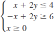
EXAMPLE 4 System of Linear Inequalities
Graph the system of linear inequalities
![]()
Solution Substitution of (0, 0) into the first inequality in (4) gives the true statement 0 ≤ 1, which implies that the graph of the solutions of x + y ≤ 1 is the half-plane below (and including) the line x + y = 1. This is the shaded blue region in FIGURE 9.4.5(a). Similarly, substituting (0, 0) into the second inequality gives the false statement 0 ≥ 4, and so the graph of the solutions of −x + 2y ≥ 4 is the half-plane above (and including) the line −x + 2y = 4. This is the shaded red region in Figure 9.4.5(b). The graph of the solutions of the system of inequalities is then the intersection of the graphs of these two solution sets. This intersection is the darker region of overlapping colors shown in Figure 9.4.5(c).
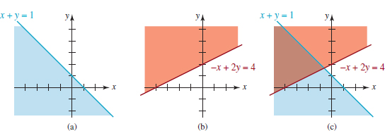
FIGURE 9.4.5 Solution set in Example 4
Often we are interested in the solutions of a system of linear inequalities subject to the restrictions that x ≥ 0 and y ≥ 0. This means that the graph of the solutions is a subset of the set consisting of the points in the first quadrant and on the nonnega-tive coordinate axes. For example, inspection of Figure 9.4.5(c) reveals that the system of inequalities (4) subject to the added requirements that x ≥ 0, y ≥ 0, has no solutions.
EXAMPLE 5 System of Linear Inequalities
The graph of the solutions of the system of linear inequalities
![]()
is the region shown in FIGURE 9.4.6(a). The graph of the solutions of

is the region in the first quadrant along with portions of the two lines and portions of the coordinate axes illustrated in Figure 9.4.6(b).

FIGURE 9.4.6 Solution set in Example 5
![]() Nonlinear Inequalities Graphing nonlinear inequalities in two variables x and y is basically the same as graphing linear inequalities. In the next example we again utilize the notion of a test point.
Nonlinear Inequalities Graphing nonlinear inequalities in two variables x and y is basically the same as graphing linear inequalities. In the next example we again utilize the notion of a test point.
EXAMPLE 6 Graph of a Nonlinear Inequality
To graph the nonlinear inequality
x2 + y2 − 4≥0
we begin by drawing the circle x2 + y2 = 4 using a solid line. Since (0, 0) lies in the interior of the circle we can use it for a test point. Substituting x = 0 and y = 0 in the inequality gives the false statement −4 ≥ 0 and so the solution set of the given inequality consists of all the points either on the circle or in its exterior. See FIGURE 9.4.7.
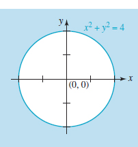
FIGURE 9.4.7 Solution set in Example 6
EXAMPLE 7 System of Inequalities
Graph the system of inequalities

Solution Substitution of the coordinates of (0, 0) into the first inequality gives the true statement 0 ≤ 4 and so the graph of y ≤ 4 − x2 is the shaded blue region in FIGURE 9.4.8 below the parabola y = 4 − x2. Note that we cannot use (0, 0) as a test point for the second inequality since (0, 0) is a point on the line y = x. However, if we use (1, 2) as a test point, the second inequality gives the true statement 2 > 1. Thus the graph of the solutions of y. x is the shaded red half-plane above the line y = x in Figure 9.4.8. The line itself is dashed because of the strict inequality. The intersection of these two colored regions is the darker region in the figure.

FIGURE 9.4.8 Solution set in Example 7
9.4 Exercises Answers to selected odd-numbered problemsbegin on page ANS-27.
In Problems 1–12, graph the given inequality.
1. x + 3y ≥ 6
2. x − y ≤ 4
3. x + 2y < −x + 3y
4. 2x + 5y > x − y + 6
5. −y ≥ 2(x + 3) − 5
6. x ≥ 3(x + 1) + y
7. y ≥ (x − 1)2
8. ![]()
9. ![]()
10. ![]()
11. ![]()
12. ![]()
In Problems 13–36, graph the given system of inequalities.
13. ![]()
14. ![]()
15. ![]()
16. ![]()
17. 
18. 
19. ![]()
20. ![]()
21. 
22. 
23. 
24. 
25. 
26. 
27. ![]()
28. ![]()
29. ![]()
30. ![]()
31. ![]()
32. 
33. ![]()
34. ![]()
35. 
36. 
In Problems 37–40, find a system of linear inequalities whose graph is the region shown in the given figure.
37. 
FIGURE 9.4.9 Region for Problem 37
38. 
FIGURE 9.4.10 Region for Problem 38
39. 
FIGURE 9.4.11 Region for Problem 39
40. 
FIGURE 9.4.12 Region for Problem 40
For Discussion
In Problems 41 and 42, graph the given inequality.
41. −1 ≤ x + y ≤ 1
42. −x ≤ y ≤ x
Project

FIGURE 9.4.13 Envelope in Problem 43
43. Ancient History and USPS Some years ago the restrictions on first-class envelope size were a bit more confusing than they are today. Consider the rectangular envelope of length x and height y shown in FIGURE 9.4.13 and the following postal regulation of November 1978:
All first-class items weighing one ounce or less and all single-piece third-class items weighing two ounces or less are subject to an extra mailing fee when the height is greater than 6
in., or the length is greater than 11
in., or the length is less than 1.3 times the height, or the length is greater than 2.5 times the height.
In parts (a)–(c) assume that the weight specification is satisfied.
(a) Using x and y, interpret the above regulation as a system of linear inequalities.
(b) Graph the region that describes envelope sizes that are not subject to an extra mailing fee.
(c) Under this regulation does an envelope of length 8 in. and height 4 in. require an extra fee?
(d) Do some research and compare the 2010 first-class regulation against the one just given.
Introduction When two rational functions, say, ![]() are added, the terms are combined by means of a common denominator:
are added, the terms are combined by means of a common denominator:

Adding numerators on the right-hand side of (1) yields the single rational expression

An important procedure in the study of integral calculus requires that we be able to reverse the process; in other words, starting with a rational expression such as (2) break it down, or decompose it, into simpler component fractions 2⁄(x + 5) and 1⁄(x + 1) called partial fractions.
![]() Terminology The algebraic process for breaking down a rational expression such as (2) into partial fractions is known as partial fraction decomposition. For convenience we will assume that the rational function P(x)⁄Q(x), Q(x) ≠ 0, is a proper fraction or proper rational expression; that is, the degree of P(x) is less than the degree of Q(x). We will also assume once again that the polynomials P(x) and Q(x) have no common factors.
Terminology The algebraic process for breaking down a rational expression such as (2) into partial fractions is known as partial fraction decomposition. For convenience we will assume that the rational function P(x)⁄Q(x), Q(x) ≠ 0, is a proper fraction or proper rational expression; that is, the degree of P(x) is less than the degree of Q(x). We will also assume once again that the polynomials P(x) and Q(x) have no common factors.
In the discussion that follows we consider four cases of partial fraction decomposition of P(x)⁄Q(x). The cases depend on the factors in the denominator Q(x). When the polynomial Q(x) is factored as a product of (ax + b)n and (ax2 + bx + c)m, n = 1, 2, …, m = 1, 2, …, where the coefficients a, b, c are real numbers and the quadratic polynomial ax2 + bx + c is irreducible over the real numbers (that is, does not factor using real numbers), the rational expression P(x)/Q(x) can be decomposed into a sum of partial fractions of the form
![]()
CASE 1: Q(x) Contains Only Nonrepeated Linear Factors
We state the following fact from algebra without proof. If the denominator can be factored completely into linear factors,
Q(x) = (a1x + b1)(a2x + b2)… (an x + bn),
where all the aix + bi, i = 1, 2, …, n are distinct (that is, no two factors are the same), then unique real constants C1, C2, …, Cn can be found such that

In practice we will use the letters A, B, C, … in place of the subscripted coefficients C1, C2, C3, …. The next example illustrates this first case.
EXAMPLE 1 Distinct Linear Factors
To decompose ![]() into individual partial fractions we make the assumption, based on the form given in (3), that the rational function can be written as
into individual partial fractions we make the assumption, based on the form given in (3), that the rational function can be written as

We now clear (4) of fractions; this can be done by either combining the terms on the right-hand side of the equality over a least common denominator and equating numerators or by simply multiplying both sides of the equality by the denominator (x − 1)(x + 3) on the left-hand side. Either way, we arrive at
![]()
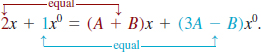
Multiplying out the right-hand side of (5) and grouping by powers of x gives
![]()
Each of the equations (5) and (6) is an identity, which means that the equality is true for all real values of x. As a consequence, the coefficients of x on the left-hand side of (6) must be the same as the coefficients of the corresponding powers of x on the right-hand side, that is,
The result is a system of two linear equations in two variables A and B:
![]()
By adding the two equations we get 3 = 4A and so we find that ![]() Substituting this value into either equation in (7) then yields
Substituting this value into either equation in (7) then yields ![]() Hence the desired decomposition is
Hence the desired decomposition is

You are encouraged to verify the foregoing result by combining the terms on the right-hand side of the last equation by means of a common denominator.
![]() A Shortcut Worth Knowing If the denominator contains, say, three linear factors such as in
A Shortcut Worth Knowing If the denominator contains, say, three linear factors such as in ![]() then the partial fraction decomposition looks like this:
then the partial fraction decomposition looks like this:
![]()
By following the same steps as in Example 1, we would find that the analog of (7) is now three equations in the three unknowns A, B, and C. The point is this: The more linear factors in the denominator the larger the system of equations we must solve. There is a procedure worth learning that can cut down on some of the algebra. To illustrate, let’s return to the identity (5). Since the equality is true for every value of x, it holds for x = 1 and x = −3, the zeros of the denominator. Setting x = 1 in (5) gives 3 = 4A, from which it follows immediately that ![]() Similarly, by setting x = −3 in (5), we obtain −5 = (−4)B or
Similarly, by setting x = −3 in (5), we obtain −5 = (−4)B or ![]()
CASE 2: Q(x) Contains Repeated Linear Factors
If the denominator Q(x) contains a repeated linear factor (ax + b)n, n > 1, then unique real constants C1, C2, …, Cn can be found such that the partial fraction decomposition of P(x)/Q(x) contains the terms
![]()
EXAMPLE 2 Repeated Linear Factors
To decompose ![]() into partial fractions we first observe that the denominator consists of the repeated linear factor x and the nonrepeated linear factor 2x − 1. Based on the forms in (3) and (8) we assume that
into partial fractions we first observe that the denominator consists of the repeated linear factor x and the nonrepeated linear factor 2x − 1. Based on the forms in (3) and (8) we assume that

Multiplying (9) by x3(2x − 1) clears it of fractions and yields
![]()
![]()
Now the zeros of the denominator in the original expression are x = 0 and ![]() If we then set x = 0 and
If we then set x = 0 and ![]() in (10), we find, in turn, that C = + and D = 16. Because the denominator of the original expression has only two distinct zeros, we can find A and B by equating the corresponding coefficients of x3 and x2 in (11):
in (10), we find, in turn, that C = + and D = 16. Because the denominator of the original expression has only two distinct zeros, we can find A and B by equating the corresponding coefficients of x3 and x2 in (11):
0 = 2A + D, 0 = −A + 2B.
![]() The coefficients of x3 and x2 on the left-hand side of (11) are both 0.
The coefficients of x3 and x2 on the left-hand side of (11) are both 0.
Using the known value of D, the first equation yields A = −D/2 = −8. The second then gives B = A/2 = −4. The partial fraction decomposition is

CASE 3: Q(x) Contains Nonrepeated Irreducible Quadratic Factors
If the denominator Q(x) contains nonrepeated irreducible quadratic factors ai x2 + bi x + ci, then unique real constants A1, A2, …, An, B1, B2, …, Bn can be found such that the partial fraction decomposition of P(x)/Q(x) contains the terms

![]() Use the quadratic formula. For either factor you will find that b2 – 4ac < 0.
Use the quadratic formula. For either factor you will find that b2 – 4ac < 0.
EXAMPLE 3 Irreducible Quadratic Factors
To decompose ![]() into partial fractions we first observe that the quadratic polynomials x2 + 1 and x2 + 2x + 3 are irreducible over the real numbers. Hence by (12) we assume that
into partial fractions we first observe that the quadratic polynomials x2 + 1 and x2 + 2x + 3 are irreducible over the real numbers. Hence by (12) we assume that
![]()
After clearing fractions in the preceding line, we find
4 x = (Ax + B)(x2 + 2x + 3) + (Cx + D)(x2 + 1)
= (A + B)x3 + (2A + B + D)x2 + (3A + 2B + C)x + (3B + D).
Because the denominator of the original fraction has no real zeros, we have no recourse except to form a system of equations by comparing coefficients of all powers of x:

Using C = −A and D = −3B from the first and fourth equations we can eliminate C and D in the second and third equations:

Solving this simpler system of equations yields A = 1 and B = 1. Hence, C = −1 and D = −3. The partial fraction decomposition is
![]()
CASE 4: Q(x) Contains Repeated Irreducible Quadratic Factors
If the denominator Q(x) contains a repeated irreducible quadratic factor (ax2 + bx + c)n, n > 1, then unique real constants A1, A2, …, An, B1, B2, …, Bncan be found such that the partial fraction decomposition of P(x)/Q(x) contains the terms

EXAMPLE 4 Repeated Quadratic Factor
Decompose ![]() into partial fractions.
into partial fractions.
Solution The denominator contains only the repeated irreducible quadratic factor x2 + 4. As indicated in (13) we assume a decomposition of the form
![]()
Clearing fractions by multiplying both sides of the preceding equality by (x2 + 4)2 gives
![]()
As in Example 3, the denominator of the original has no real zeros and so we must solve a system of four linear equations for A, B, C, and D. To that end we rewrite (14) as
0x3 + 1x2 + 0x + 0x0 = Ax3 + Bx2 + (4A + C)x + (4B + D)x0
and compare coefficients of like powers (match the colors) to obtain

From this system we find that A = 0, B = 1, C = 0, and D = −4. The required partial fraction decomposition is then
![]()
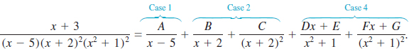
EXAMPLE 5 Combination of Cases
Determine the form of the decomposition of ![]()
Solution The denominator contains a single linear factor x − 5, a repeated linear factor x + 2, and a repeated irreducible quadratic factor x2 + 1. By Cases 1, 2, and 4 the assumed form of the partial fraction decomposition is
NOTES FROM THE CLASSROOM

We assumed throughout the foregoing discussion that the degree of the numerator P(x) was less than the degree of the denominator Q(x). If, however, the degree of P(x) is greater than or equal to the degree of Q(x), then P(x)/Q(x) is an improper fraction. We can still do partial fraction decomposition but the process starts with long division until a polynomial quotient and a proper fraction is attained. For example, long division gives

Then by using Case + we finish the problem with the decomposition of the proper fraction term in the last equality:
![]()
See Problems 25–30 in Exercises 9.5.
9.5 Exercises Answers to selected odd-numbered problems begin on page ANS–28.
In Problems 1–24, find the partial fraction decomposition of the given rational expression.
1. ![]()
2. 
3. ![]()
4. ![]()
5. 
6. ![]()
7. ![]()
8. ![]()
9. ![]()
10. ![]()
11. ![]()
12. 
13. ![]()
14. ![]()
15. ![]()
16. ![]()
17. ![]()
18. 
19. ![]()
20. ![]()
21. 
22. ![]()
23. ![]()
24. ![]()
In Problems 25–30, first use long division followed by partial fraction decomposition.
25. ![]()
26. 
27. ![]()
28. ![]()
29. ![]()
30. ![]()
A. Fill in the Blanks__________________________________
In Problems 1-10, fill in the blanks.
1. The linear system

is consistent for b = _______.
2. ![]()
3. If  then x = _______.
4. By Cramer’s Rule the solution of the linear system
![]()
α ≠ 0, β ≠ 0, is _______.
5. The graph of a single linear inequality in two variables represents a _______ in the plane.
6. A solution of the nonlinear system

is _______.
7. The solution of the linear system

is _______.
8. If the system of two linear equations in two variables has an infinite number of solutions, then the equations are said to be _______.
9. If the graph of y = ax2 + bx passes through (1,1) and (2,1), then a = _______ and b = _______.
10. The graph of the nonlinear system of inequalities
lies in the _______ quadrant.
B. True/False ____________________________________
In Problems 1-10, answer true or false.
1. The graphs of 2x + 7y = 6 and x4 + 8xy − 3y6 = 0 intersect at (−4, 2). _______
2. The homogeneous linear system

possesses only the zero solution (0,0,0) _______.
3. The nonlinear system

always has two solutions when m ≠ 0 and k > 0. _______
4. If the determinant of the coefficients in a system of three linear equations and three variables is 0, then Cramer’s Rule indicates that the system has no solution. _______
5. The nonlinear systems

are equivalent. _______
6. (1,−2) is a solution of the inequality 4x − 3y + 5 ≤ 0. _______
7. The origin is in the half-plane determined by 4x − 3y < 6. _______
8. The system of linear inequalities
![]()
has no solutions. _______
9. The system of nonlinear equations
![]()
has exactly three solutions. _______
10. The form of the partial-fraction decomposition of ![]()
C. Review Exercises ______________________________
In Problems 1–14, find all real solutions of the given system of equations.
1. 
2. 
3. 
4. ![]()
5. ![]()
6. ![]()
7. ![]()
8. 
9. ![]()
10. ![]()
11. ![]()
12. ![]()
13. ![]()
14. ![]()
15. Playing with Numbers In a two-digit number, the units digit is 1 greater than 3 times the tens digit. When the digits are reversed, the new number is 45 more than the old number. Find the old number.
16. Lengths A right triangle has an area of 24 cm2. If its hypotenuse has a length of 10 cm, find the lengths of the remaining two sides of the triangle.
17. Got a Wire Cutter? A wire 1 m long is cut into two pieces. One piece is bent into a circle and the other piece is bent into a square. The sum of the areas of the circle and the square is ![]() What are the lengths of the sides of the square and the radius of the circle?
What are the lengths of the sides of the square and the radius of the circle?
18. Coordinates Find the coordinates of the point P of intersection of the line and the parabola shown in FIGURE 9.R.1.

FIGURE 9.R.1 Graphs for Problem 18
In Problems 19–22, find the partial fraction decomposition of the given rational expression.
19. 
20. ![]()
21. ![]()
22. ![]()
In Problems 23–28, graph the given system of inequalities.
23. 
24. 
25. 
26. 
27. 
28. 
29. In words, describe the graph of the inequality 1 ≤ x − y ≤ 4.
30. Using the equations y = 9 − x2 and y = 4 − x2, give:
(a) a system of two inequalities that has no solution,
(b) a system of two inequalities for which (1, 9) is a member of the solution set.
In Problems 31–34, use the functions y = x2 and y = 2 − x to form a system of inequalities whose graph is given in the figure.
31. 
FIGURE 9.R.2 Graphs for Problem 31
32. 
FIGURE 9.R.3 Graphs for Problem 32
33. 
FIGURE 9.R.4 Graphs for Problem 33
34. 
FIGURE 9.R.5 Graphs for Problem 34
In Problems 35–40, match one of the systems of equations given in (a)–(f) with the graphs given in the figure.
(a) ![]()
(b) ![]()
(c) ![]()
(d) ![]()
(e) ![]()
(f) ![]()
35. 
FIGURE 9.R.6 Graphs for Problem 35
36. 
FIGURE 9.R.7 Graphs for Problem 36
37. 
FIGURE 9.R.8 Graphs for Problem 37
38. 
FIGURE 9.R.9 Graphs for Problem 38
39. 
FIGURE 9.R.10 Graphs for Problem 39
40. 
FIGURE 9.R.11 Graphs for Problem 40
41. Give a system of inequalities whose graph is given in FIGURE 9.R.12.
42. Give an example of a nonlinear system of two equations that has four solutions but the graphs of the equations intersect at only two points.

FIGURE 9.R.12 Graphs for Problem 41