
This chapter presents the basics of business intelligence (BI). If you're an experienced data warehouse expert, you may wish to skip this chapter, except for the section that introduces SharePoint 2010 BI concepts at the end. But, since a huge part of our audience will be SharePoint experts, not data warehouse experts, we felt it necessary to include the fundamentals of data warehousing in this book. While we don't intend to cover every detail, we'll include what you need to know to get through the book, and refer you to other resources for advanced concepts.
Effective decision-making is the key to success, and the key to making effective decisions is appropriate and accurate information. Data won't do you much good if you can't get any intelligent information from it, and to do that, you need to be able to properly analyze the data. There's a lot of information embedded in the data in various forms and views that can help organizations and individuals create better plans for the future. We'll start here with the fundamentals of drilling down into data—how to do it and how you can take advantage of it.
I couldn't resist including a picture here that highlights the benefits of BI (see Figure 1-1). This drawing was presented by Hasso Plattner of the Hasso Plattner Institute for IT Systems at the SIGMOD Keynote Talk. (SIGMOD is the Special Interest Group on Management of Data of the Association for Computing Machinery.)

By the end of this chapter, you'll learn about:
The essentials of BI
The OLAP system and its components
SQL Server 2008 BI Tools
SharePoint 2010 BI Components
You'll need a basic understanding of databases and the relevant tools to get the most out of the topics in this book. You'll also need the software listed here:
SharePoint Server 2010 Enterprise Edition
SQL Server 2008 R2 Developer Edition and its BI tools, BIDS (Business intelligence development studio 2008)
SQL Server 2008 R2 Update for Developers Training Kit (June 2010 Update), available for download at
http://www.microsoft.com/downloads/details.aspx?FamilyID=fffaad6a-0153-4d41-b289-a3ed1d637c0d&displaylang=enAdventureWorks DB for SQL Server 2008R2, available for download at
http://msftdbprodsamples.codeplex.com/releases/view/45907Visual Studio 2010 Professional Edition, trial version available for download at
http://www.microsoft.com/visualstudio/en-us/products/2010-editions/professionalMicrosoft SharePoint Designer 2010, available for download at
http://www.microsoft.com/downloads/details.aspx?FamilyID=d88a1505-849b-4587-b854-a7054ee28d66&displaylang=enIf you'd prefer using Express editions of Visual Studio and SQL Server instead of the full versions, you can download them from
http://www.microsoft.com/express/.
Chances are you've seen the recommendations pages on sites such as Netflix, Wal-Mart, and Amazon. On Netflix, for example, you can choose your favorite genre, then the movies to order or watch online. Next time you log in, you'll see a "Movies you'll love" section with several suggestions based your previous choices. Clearly, there's some kind of intelligence-based system running behind these recommendations. Now, don't worry about what technologies the Netflix web application is built on. Let's just try to analyze what's going on behind the scenes. First, since there are recommendations, there must be some kind of tracking mechanism for your likes and dislikes based on your choices or on the ratings you provide. Second, recommendations may be based on other users' average ratings minus yours for a given genre. Each user provides enough information to let Netflix drill down, aggregate, and otherwise analyze different kinds of scenarios. This analysis can be either simple or complex depending on many other factors, including total number of users, movies watched, genre, ratings, and so on—with endless possibilities.
Now consider a related but not so similar example—your own online banking information. The account information in your profile is presented in various charts on various timelines, and so forth, and you can use different tools to add or alter information to see how your portfolio might look in the future.
Now think along the same lines, but this time about a big organization with millions of records that can be explored to give CIOs or CFOs a picture of their assets, revenues, sales, and so forth. It doesn't matter if the organization is financial, medical, technical, or whatever, or what the details of information are. There's no limit for data in how it can be drilled down and understood. In the end, it boils down to one thing—using business intelligence to enable effective decision making.
Let's get started on our explorations of the basics and building blocks of business intelligence.
Just about any kind of business will benefit from having appropriate, accurate, and up-to-date information in order to make key decisions. The question is, how do you get this information when the data is tightly coupled with business—and is in use. In general, you need to think about questions such as:
How can you drill down into tons of information, aggregate that information, and perform mathematical calculations to analyze it?
How can you use such information to understand what's happened in the past as well as what's happening now, and thereby build better solutions for future?
Here are some typical and more specific business-related questions you might have to answer.
What are the newly created accounts this month?
Which new users joined this quarter?
Which accounts have been removed this year?
How many vehicles have we sold this year and what's the new inventory?
How many issues have been addressed this week in the command center?
What is the failure rate of products in this unit?
What are the all-time top 10 stocks?
Can you rank these employees in terms of monthly sales?
Is it possible to run statistical analysis on existing data?
What kind of system could provide the means to answer these questions? A comprehensive business intelligence system is a powerful mechanism for digging into, analyzing, and reporting on your data.
Note
Business intelligence is all about decisions made effectively with accurate information in timely manner.
Data always has a trend or a paradigm. When you're looking at the data, you might begin to wonder, "What if...." To answer this question, you need the business intelligence mechanism. Understanding the basics of BI or data warehouse modeling helps you achieve accurate results.
Every industry, organization, enterprise, firm, or even individual has information stored in some format in databases or files somewhere. Sometimes this data will just be read, and sometimes it needs to be modified and provide instant results. In such cases, one significant factor is the size of the data. Databases that yield instant results by adding, editing, or deleting information deal with transactional data. Such information needs a quick turnaround from the applications. In such cases, users seek or provide information via the UI or another source, and the result of any subsequent read, publish, edit, or even delete must happen instantly. Transaction results must also be delivered instantly, without any latency. A system that can deliver such instant results usually is based on the model called Online Transaction Processing or just OLTP.
Data in the OLTP model is relational, and it is normalized according to database standards—such as the third or fourth normal form. An important factor in the OLTP model is that data doesn't repeat in any fashion and hence it is arranged into more than one table. In this way, transactions involve fewer tables and columns, thus increasing performance. There are fewer indexes and more joins in this model, and the tables will hold the key information.
Figure 1-2 shows a basic OLTP system.

Note
We strongly recommend you download and install the AdventureWorks sample database. You'll get the most out of this chapter and the others if you can follow along.
OLTP is not meant for slicing and dicing the data, and it's definitely not meant to be used to make key decisions based on the data. OLTP is real-time and it's optimized for performance during Read/Write operations specifically for a faster response.
Now take a look at Figure 1-3. Notice how information is limited or incomplete. You wouldn't be able to tell what the numbers or codes are for various columns. To get more information on these values, you'd need to run a query that would join this table with others, and the query could become bigger and bigger as the number of relational tables increases.

On the other hand, it would be very easy to query the table if it were a little bit denormalized and had some data pre-populated, as shown in Figure 1-4. In this case, the number of joins would be reduced, thereby shortening the T-SQL query. This would simplify the query and improve the performance. However the performance depends on the efficiency of indexing and note that denormalizing the tables cause excessive I/O.

Warning
As you can see in Figure 1-4, the T-SQL query would be simplified, but denormalized tables can cause excessive I/O because they contain fewer records on a page. It depends on the efficiency of the indexing. The data and indexes also consume more disk space than normalized data.
You might ask, why can't I simply run these queries on my OLTP database without worries about performance? Or create views? Simply put, OLTP databases are meant for regular transactions that happen every day in your organization. These are real-time and current at any point of time, which makes OLTP a desirable model. However, this model is not designed to run powerful analysis on these databases. It's not that you can't run formulas or aggregates, it's that the database might have been built to support most of the applications running in your organization and when you try to do the analysis, these applications take longer to run. You don't want your queries to interfere with or block the daily operations of your system.
Note
To scale operations, some organizations split an OLTP database into two separate databases (i.e., they replicate the database). One database handles only write operations while the other is used for read operations on the tables (after the transactions take place). Applications manage through code the data to write to one database and to read for presentation from another database. This way, transactions take place on one database and analysis can happen on the second. This may not be suitable for every organization.
So what can we do? Archive the database! One way that many organizations are able to run their analysis on an OLTP databases is to simply take periodic backups or archive the real-time database, and then run their queries on the disconnected-mode (non-real-time) data.
Note
A database that has been backed up and repurposed (copied) for running analysis might require a refresh as the original source database might have had data updated or values changed.
Good enough? Still, these OLTP databases are not meant for running analysis. Suppose you have a primary table consisting of information for one row in four different normalized tables, each having eight rows of information, the complexity is 1×4×8×8. But what if you're talking about a million rows? Imagine what might happen to the performance of this query!
Note
The data source for your analysis need not be OLTP. It can be an Excel file, a text file, a web service, or information stored in some other format.
We must emphasize that we are not saying that OLTP doesn't support analysis. All we are saying is that OLTP databases are not designed for complex analysis. What we need is a non-relational and non-live database where such analysis can be freely run on data to support business intelligence.
To tune your database to the way you need to run analysis on it needs some kind of cleaning and rearranging of data, which can be done via a process known as Extract, Transform, and Load (ETL). That simply means data is extracted from the OLTP databases (or any other data sources), transformed or cleaned, and loaded into a new structure. Then what? What comes next?
The next question to be asked is, even if we have ETL, to what system should the data be extracted, transformed, and loaded? The answer: It depends! As you'll see, the answer to lots of things database-related is "It depends!"
To analyze our data, what we need is a mechanism that can make it feasible to drill down, run an analysis, and understand the data. Such results can provide tremendous benefits in making key decisions. Moreover, they give you a window that may display the data in a brand-new way. We already mentioned that the mechanism to pull the intelligence from your data is BI, but the system to facilitate and drive this mechanism is the OLAP structure, the Online Analytical Processing system.
The key term in the name is analytical. OLAP systems are read-only (though there can be exceptions) and are specifically meant for analytical purposes, which facilitates most of the needs of BI. When we say a read-only database, it's essentially a backup copy of the real-time OLTP database, or more likely a partial copy of an entire OLTP database.
In contrast with OLTP, OLAP information is considered historical, which means that though there may be batch additions to the data, it is not considered up-to-the-second data. Data is completely isolated and is meant for performing various tasks, such as drilldown and the like. Information is stored in fewer tables and so queries perform much faster since they involve fewer joins.
Note
OLAP systems relax normalization rules by not following the third normal form.
Table 1-1 compares OLTP and OLAP systems.
Table 1-1. OLTP vs. OLAP
Online Transaction Processing System | Online Analytical Processing System |
|---|---|
|
|
You're probably already wondering how you can take your OLTP database and convert it to OLAP database so you can run some analysis on it. Before you run off to find out the solution, it's important to know a little more about OLAP and its structure.
Data cubes are more sophisticated OLAP structures that will solve the above concern. Despite the name, cubes are not limited to a cube structure. The name is inherited just because it has more dimensions. Don't visualize cubes as only 3-dimensional or symmetric; cubes are used for their multidimensional value.
A simple cube can have only three dimensions, such as those shown in Figure 1-5 where X is Products, Y is Region, and Z is Time.

With a cube like the one in Figure 1-5, you can find out product sales in a given time frame. This cube uses Product Sales as facts with the Time dimension.
Facts (also called measures) and dimensions are integral parts of cubes. Data in cubes is accumulated as facts and aggregated against a dimension. A data cube is multi-dimensional and thus can deliver information based on any fact against any dimension in its hierarchy.
Dimensions can be described by their hierarchies, which are essentially parent-child relationships. If dimensions are key factors of cubes, hierarchies are key factors of dimensions. In the hierarchy of the Time dimension, for example, you might find Yearly, Half-yearly, Quarterly, Monthly, Weekly, and Daily levels. These become the facts or members of the dimension.
In a similar vein, geography might be described like this:
Country
Regions
East
West
North
South
States
Counties
Figure 1-6 shows a multi-dimensional cube.

Now imagine cubes with multiple facts and dimensions, each dimension having its own hierarchies across each cube, and all these cubes connected together. The information residing inside this consolidated cube can deliver very useful, accurate, and aggregated information. You can drill down into the data of this cube to the lowest levels.
However, earlier we said that OLAP databases are denormalized. Well then, what happens to the tables? Are they not connected at all and just work independently?
Clearly, you must have the details of how your original tables are connected. If you want to convert your normalized OLTP tables into denormalized OLAP tables, you need to understand your existing tables and their normalized form in order to design the new mapping for these tables against the OLAP database tables you're planning to create.
In order to plan for migrating OLTP to OLAP, you need to understand a more about OLAP internals. OLAP structures its tables in its own style, yielding tables that are much cleaner and simpler. However, it's actually the data that makes the tables clean and simple. To enable this simplicity, the tables are formed into a structure (or pattern) that can be depicted visually as a star. Let's take a look at how this so-called star schema is formed and at the integral parts that make up the OLAP star schema.
OLAP data tables are arranged to form a star. Star schemas have two core concepts: facts and dimensions. Facts are values or calculations based on the data. They may be just numeric values. Here are some examples of facts:
Dell US Eastern Region Sales on Dec 08, 2007 are $1.7M.
Dell US Northern Region Sales on Dec 08, 2007 are $1.1M.
Average daily commuters in Loudoun County Transit in Jan. 2010 are 11,500.
Average daily commuters in Loudoun County Transit in Feb. 2010 are 12,710.
Dimensions are the axis points, or ways to view facts. For instance, using the multidimensional cube in Figure 1-6 (and assuming it relates to Wal-Mart), we can ask
What is Wal-Mart's sales volume for Date mm/dd/yyyy? Date is a dimension.
What is Wal-Mart's sales volume in the Eastern Region? Region is a dimension.
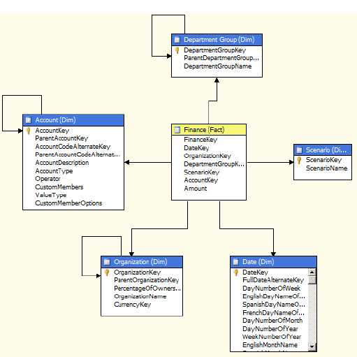
Values around the cube that belong to a dimension are known as members. In Figure 1-6, examples of members are Eastern (under the Region dimension), Prod 2 (under Products) and Yearly (under Time). You might want to aggregate various facts against various dimensions. Generating and obtaining a star schema is very simple using SQL Server Management Studio (SSMS). You can create a new database diagram by adding more tables from the AdventureWorks database. SSMS will link related tables and form a star schema as shown in Figure 1-7.
Note
OLAP and star schemas are sometimes spoken of interchangeably.
In Figure 1-7, the block in center is the fact table and those surrounding the center block are dimensions. This layout—a fact table in the center surrounded by the dimensions—is what makes a star schema.
OLAP data is in the form of aggregations. We want to get from OLAP information such as:
The volume of sales for Wal-Mart last month.
The average salaries paid to employees this year.
A statistical comparison of our own company details historically, or a comparison against other companies.
and so on.
Note
Another model similar to the star schema is the snowflake schema, which is formed when one or more dimension table is joined to another dimension table(s) instead of a fact table. This results in reference relationships between dimensions, or in other words they are normalized.
So far so good! Although the OLAP system is designed with these schemas and structures, it's still a relational database. It still has all the tables and relations as an OLTP database, which means that querying from these OLAP tables might still have performance issues and thus creates a bit of concern in aggregation.
Note
Aggregation is nothing but summing or adding data or information on a given dimension.
It is the structure of the cubes that solves those performance issues; cubes are very efficient and fast in providing information. The next question then is how to build these cubes and populate them with data. Needless to say, data is an essential part of your business and, as we've noted, typically exists in an OLTP database. What we need to do is retrieve this information from the OLTP database, clean it up, and transfer the data (either in its entirety or only what's required) to the OLAP cubes. Such a process is known as Extract, Transform, and Load (ETL).
Note
ETL tools can extract information not only from OLTP databases, but also from different relational databases, web services, file systems, or various other data sources.
You will learn about some of the ETL tools later in this chapter. We'll start by taking a look at data transfer from an OLTP database to an OLAP database using ETL, at a very high level. But we can't just jump right in and convert these systems. Be warned, ETL requires some preparations, so we'd better discuss those now.
The ETL process pulls data from various data sources that can be in a form as simple as a flat text file or as complex as a SQL Server or Oracle database. Moreover, the data may come from different sources of unknown formats, as when an organization has merged with another. Or it could be an even worse scenario, where not only the data schemas are different but the data sources are completely be different as well. There might be different databases such as SQL, Oracle, or DB2, or, for that matter, even flat files and xml files. And these data sources may very well be real-time OLTP databases that can't be directly accessed to retrieve information. Furthermore, the data likely needs to be loaded on a periodic basis as updates happen in real time—probably every second. Now imagine that this involves terabytes of data. How much time would it take to copy the data from one system and load into another? As you can tell, this is likely to be a very difficult situation.
All of these common issues essentially demand an area where you can happily carry out all your operations—a staging or data preparation platform. How would you take advantage of a staging environment? Here are the tasks you'd perform:
Identify the data sources and prepare a data map for the existing (source) tables and entities.
Copy the data sources to the staging environment or use a similar process to achieve this. This step essentially isolates the original data source.
Identify the data source tables, their formats, column types, etc.
Prepare for common ground; that is, make sure mapping criteria is in sync with the destination database.
Remove unwanted columns.
Clean column values. You definitely don't want unwanted information; this brings in less data but enough to run the analysis.
Prepare, plan, and schedule for reloading the data from the source and going through the entire cycle of mapping.
Once you are ready, use proper ETL tools to migrate the data to destination.
Let's begin with a simple flow diagram, shown in Figure 1-8, which shows everything put together very simply. Think about the picture in terms of rows and columns, as we have three rows—for system, language used, and purpose, and 2 columns—one for OLTP and the other for OLAP.
On OLTP databases you use the T-SQL language to perform the transactions, while for OLAP databases you use MDX queries instead to parse the OLAP data structures (which, in this case, are cubes). And, finally, you use OLAP/MDX for BI analysis purposes.

What is ETL doing in Figure 1-8? As we noted, ETL is the process used to migrate an OLTP database to an OLAP database. Once the OLAP database is populated with the OLTP data, we use MDX queries and run them against the OLAP cubes to get what need (the analysis).
Now that you understand the transformation, let's take a look at MDX scripting and see how you can use it to achieve your goals.
MDX stands for Multidimensional Expressions. It is an open standard used to query information from cubes. Here's a simple MDX query (running on the AdventureWorks database):
select [Measures].[Internet Total Product Cost] ON COLUMNS,
[Customer].[Country] ON ROWS
FROM [AdventureWorks]
WHERE [Sales Territory].[North America]
MDX can be a very simple select statement as shown above, which consists of the select query and choosing columns and rows, much like a traditional SQL select statement. In a nutshell, it's like this:
Select x, y, z from cube where dimension equals a.Sound familiar?
Let's look at the MDX statement more closely. The query is retrieving information from the measure "Internet Total Product Cost" against the dimension "Customer Country" from the Cube "AdventureWorks." Furthermore, the where clause is on the "Sales Territory" Dimension, as we are intrested in finding the Sales in North America.
Note
Case sensitivity for columns and rows is not mandatory. Also, you can use 0 and 1 as ordinal positions for columns and rows respectively. If you extend the ordinal positions beyond 0 and 1, MDX will return the multidimensional cube.
MDX queries are not so different from SQL queries except that MDX used to query an analysis cube. It has all the rich features, similar syntax, functions, support for calculations, and more. The difference is that SQL retrieves information from tables that basically results in a two-dimensional view. In contrast, MDX can query from a cube and deliver mutidimensional views.
Go back and take a look at Figure 1-6, which shows sales (fact) against three dimensions: Product, Region, and Time. This means you can find the sales for a given product in a given region at a given time. This is simple. Now suppose you have regions splitting the US into North, East, West and South, and the time frame further classified as Yearly, Quarterly, Monthly, and Weekly. All of these elements serve as filters, allowing you to retrieve the finest aggregated information about the product. Thus a cube can range from a simple 3-dimensional one to a complex hierarchy where each dimension can have its own members or attributes or children. You need a very clear understanding of these fundamentals in order to write efficient MDX queries.
In a multidimensional cube, you can either call the entire cube a cell or count each cube as one cell. A cell is built with dimensions and members.
Using our example cube, if you need to retrieve the sales value for a product, you'd do it as
(Region.East, Time.[Quarter 4], Product.Prod1)
Notice that squarebrackets—[ ]—are used when there's a space in the dimension/member.
Looks easy, yes? But what if you need just a part of the cube value and not the whole thing? Let's say you need just prod1 sales in the Eastern region. Well that's definitely a valid constraint. To address this, you use tuples in a cube.
A tuple is an address within the cube. You can define a tuple based on what you need. It can have one or more dimensions and one measure as a logical group. For instance, if we use the same example, data related to the Eastern Region during the fourth Quarter can be called one tuple. So
(Region.East, Time.[Quarter 4], Product.Prod1)
is a good example of a tuple. You can design as many as tuples you need within the limits of dimensions.
A set is a group of zero or more tuples. Remember that you can't use the terms tuples and sets interchangeably. Suppose you want two different areas in a cube or two tuples with different measures and dimensions. That's where you use a set (see Figure 1-9).
For example, if (Region.East, Time.[Quarter 4], Product.Prod1) is one of your tuples, and (Region.East, Time.[Quarter 1], Product.Prod2) is the second, then the set that comprises these two tuples looks like this:
{(Region.East, Time.[Quarter 4], Product.Prod1), (Region.East, Time.[Quarter 1],
Product.Prod2) }
Note
When you create MDX queries, it's always good to include comments that provide sufficient information and make logical sense. You can write single-line comments by using either "//" or "—" or multiline comments using"/*...*/".
For more about advanced MDX queries, built-in functions and their references, please consult the book Smart Business Intelligence Solutions with Microsoft SQL Server 2008, available for purchase at microsoft.com/learning/en/us/book.aspx?ID=12663&locale=en-us.
Table 1-2 gives an overview of the database models and their entities, query languages, and the tools used to retrieve information from them.
Table 1-2. Database models
Nature of usage | Transactional (R/W) Add, Update, Delete | Analytics (R) Data Drilldown, Aggregation |
|---|---|---|
Type of DB | OLTP | OLAP |
Entities | Tables, Stored Procedures, Views etc. | Cubes, Dimensions, Measures, etc. |
Query Language(s) | MDX | |
Tools | SQL Server 2005 (or higher), SSMS | SQL Server 2005 (or higher), SSMS, BIDS, SSAS |
Before proceeding, let's take a look at some more BI concepts.
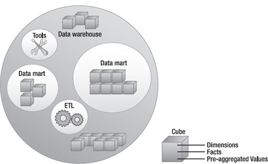
You can now visualize how big a cube can become, with infinite dimensions and facts. A data warehouse is a combination of cubes. It is how you structure enterprise data. Data warehouses are typically used at huge organizations for aggregating and analyzing their information.
Since cubes are integral parts of a data warehouse, it's evident that a data warehouse comprises both relational and disconnected databases. Data warehouses are a consolidation of many other small slices (as shown in Figure 1-10) that includes data marts, tools, data sources, and ETL.
A data mart is a baby version of the data warehouse. It also has cubes embedded in it, but you can think of a data mart as a store on Main Street and a data warehouses as one of those huge, big-box shopping warehouses. Information from the data mart is consolidated and aggregated into the data warehouse database. You have to regularly merge data from OLTP databases into your data warehouse on a schedule that meets your organization's needs. This data is then extracted to the data marts, which are designed to perform specific functions.
Note
Data marts can run independently and need not be a part of a data warehouse. They can be designed to function as autonomous structures.
Consolidating data from a data mart into a data warehouse needs to be performed with utmost care. Consider a situation where you have multiple data marts following different data schemas and you're trying to merge information into one data warehouse. It's easy to imagine how data could be improperly integrated, which would become a concern for anyone who wanted to run analysis on this data. This creates the need to use conformed dimensions (refer to http://data-warehouses.net/glossary/conformeddimensions.html for more details). As we mentioned earlier, areas or segments where you map the schemas and cleanse the data are sometimes known as staging environments. These are platforms where you can check consistency and perform data-type mapping, cleaning, and of course loading the data from the data sources. There could definitely be transactional information in each of the data marts. Again, you need to properly clean the data and identify only the needed information to migrate from these data marts to the data source.
Both decision support systems and data mining are accomplished using OLAP. While a decision support system gives you the facts, data mining provides the information that leads to prediction. You definitely need both of these as one lets you get accurate, up-to-date information whereas the other leads to questions that can provide intelligence for making future decisions (see Figure 1-11). For example, decision support provides accurate information such as "Dell stocks rose by 25 percent last year." That's precise information. Now if you pick up Dell's sales numbers from last 4 or 5 years, you can see the growth rate of Dell's annual sales. Using these figures, you might predict what kind of sales Dell would make next year. That's data mining.
Note
Data mining leads to prediction. Prediction leads to planning. Planning leads to questions such as "What if?" These are the questions that help you avoid failure. Just as you use MDX to query data from cubes, you can use the DMX (Data Mining Extensions) language to query information from data mining models in SSAS.

Now let's get to some real-time tools. What you need are the following:
Note
Installing SQL Server 2008 R2 with all the necessary tools is beyond the scope of this book. We recommend you go to Microsoft's SQL Server installation page at msdn.microsoft.com/en-us/library/bb500469.aspx for details on installation and administration.
SSMS is not something new to developers. You've probably used this tool in your day-to-day activities or at least for a considerable period during any development project. Whether you're dealing with OLTP databases or OLAP, SSMS plays a significant role, and it provides a lot of the functionality to help developers connect with OLAP databases. Not only can you run T-SQL statements, you can also use SSMS to run MDX queries to extract data from the cubes.
SSMS makes it feasible to run various query models, such as the following:
Database Engine Query: executes T-SQL, XQuery, and sqlcmd scripts.
Analysis Services MDX Query: executes MDX queries on a OLAP database.
Analysis Services DMX Query: executes DMX queries on a OLAP database.
Analysis Services XMLA Query: executes XMLA language queries on a OLAP database.
SQL Server Compact Query: executes queries of the SQL Server Compact database.
Figure 1-12 shows that the menus for these queries can be accessed in SSMS.

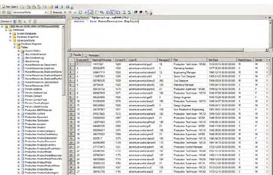
Figure 1-13 shows an example of executing a new query against an OLTP database.
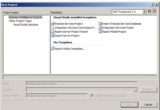
While Visual Studio is the developer's rapid application development tool, SQL Server Business Intelligence Development Studio (BIDS) 2008 is the equivalent development tool for the database developer (see Figure 1-14). BIDS looks like Visual Studio but it supports only a limited set of templates:
Analysis Services Project: The template used to create cubes, measures, and dimensions, and other related objects.
Integration Services Project: The template used to perform ETL operations.
Import Analysis Services Database: The template for creating an analysis services project based on a analysis services database.
Integration Services Connections Project Wizard: Wizard for creating new package with connections for various data sources.
Report Server Project Wizard: Wizard that facilitates creation of reports from a data source and provides options to select various layouts, etc.
Report Model Project: The template used to create report models based on a SQL Server database.
Report Server Project: The template for authoring and publishing reports.
As discussed earlier, data needs to be extracted from the OLTP databases, cleaned, and then loaded into OLAP in order to be used for business intelligence. You can use the SQL Server Integration Services (SSIS) tool to accomplish this. This section will run through various steps detailing how to use Integration Services and how it can be used as an ETL tool.
SSIS is very powerful. You can use it to extract data from any source that includes a database, a flat file, or an xml file, and you can load that data into any other destination. In general, you have a source and a destination, and they can be completely different systems. A classic example of where to use SSIS is when companies merge and they have to move their databases from one system to another, which includes the complexity of having mismatches in the columns, etc. The beauty of SSIS is that it doesn't necessarily use a SQL Server database.
Note
SSIS is considered to be the next generation of Data Transformation Service (DTS), which shipped with SQL Server versions prior to 2005.
The important elements of SSIS packages are control flows, data flows, connection managers, and event handlers. Let's look at some of the features of SSIS in detail, and we'll demonstrate how simple it is to import information from a source and export it to a destination.
Since we will be working with the AdventureWorks database here, let's pick some its tables, extract the data, and then import the data back to another database or a file system.
Open SQL Server BIDS and from the File menu, choose New, then select New Project. From the available Project Types, choose Business Intelligence Projects and from the Templates, choose Integration Services Project. Provide necessary details (such as Name, Location, and Solution Name) and click OK.
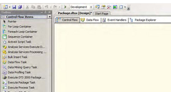
Once you create the new project, you'll land on the Control Flow screen as shown in Figure 1-15. When you create an SSIS package, you get a lot of tools in the toolbox pane that is categorized by context based on selected design window or views. There are four views namely Control Flow, Data Flow, Event Handlers and Package Explorer. Here below we will discuss two main views, the Data Flow and the Control Flow:
Data Flow
Data Flow Sources (e.g., ADO.NET Source, to extract data from a database using a .NET provider; Excel Source, to extract data from an Excel workbook; Flat File Source, to extract data from flat files, and so on).
Data Flow Transformations (e.g., Aggregate, to aggregate values in the dataset; Data Conversion, to convert columns to different data types and add columns to the dataset; Merge, to merge two sorted datasets; Merge Join, to merge two datasets using join; Multicast, to create copies of the dataset and so on).
Data Flow Destinations (e.g., ADO.NET destination, to write into a database using an ADO.NET provider; Excel Destination, to load data into a Excel workbook; SQL Server Destination, to load data into SQL Server database and so on).
Based on the selected data flow tasks, event handlers can be built and executed in the Event Handlers view.
Control Flow
Control Flow Items (e.g., Bulk Insert Task, to copy data from file to database; Data Flow Task, to move data from source to destination while performing ETL; Execute SQL Task, to execute SQL queries; Send Mail Task, to send email, and so on).
Maintenance Plan Tasks (e.g., Back Up Database Task, to back up source database to destinations files or tapes; Execute T-SQL Statement Task, to run T-SQL scripts; Notify Operator Task, to notify SQL Server Agent operator and so on).
Let's now see how to import data from a system and export it to another system.
Launch the Import and Export Wizard from the Solution Explorer as shown in Figure 1-16.
Right-click on SSIS Packages and select the SSIS Import and Export Wizard option.
Note
Another way to access the Import and Export Wizard is from C:Program FilesMicrosoft SQL Server100DTSBinnDTSWizard.exe.

Here are the steps to import from a source to a destination:
Click Next on the Welcome screen.
From the Choose a Data Source menu item, you can select various options, including Flat File Source. Select "SQL Server Native Client 10.0" in this case.
Choose the available server names from the drop-down or enter the name you prefer.
Use Windows Authentication/SQL Server Authentication.
Choose the source database. In our case, select the "AdventureWorks" database.
Next, choose the destination options and in this case select "Flat File Destination".
Choose the destination file name and set the format to "Delimited".
Choose to "Copy data from one or more tables or views" from the "Specify Table Copy or Query" window.
From the Flat File Destination window, click on "Edit mappings", leave the defaults to "Create destination file", and click on OK.
Click Finish, then click Finish again to complete the Wizard.
Once execution is complete, you'll see a summary displayed. Click Close. This step would create the .dtsx file and you need to finally run the package once to get the output file.
Importing can also be done by using various data flow sources and writing custom event handlers. Let's do it step-by-step now:
PROBLEM CASE
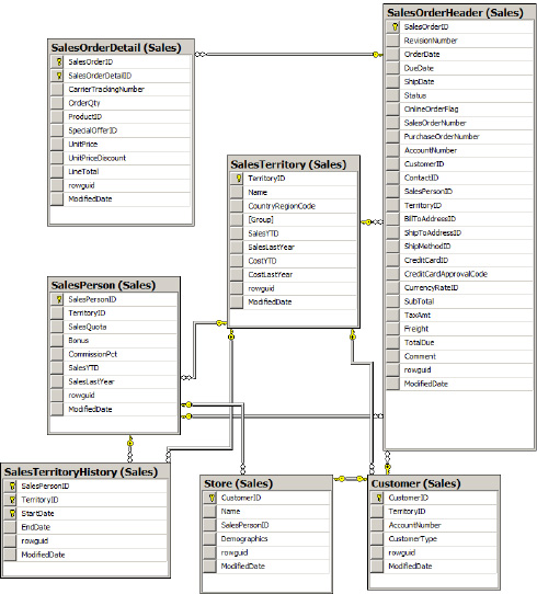
The Sales data from the AdventureWorks database consists of more than seven tables but for simplicity let's consider the seven tables displayed in Figure 1-17. Now, you need to retrieve the information from these seven tables, extract the data, clean some of the data or drop the columns that aren't required, and then load the desired data into another data source—a flat file or database table. You might also want to extract data from two different data sources and merge it into one.
Here's how to accomplish our goals:
Open BIDS and from the File menu choose New, then select New Project. From the available project types choose Business Intelligence Projects and from the Templates choose Integration Services Project. Provide necessary details (such as Name, Location, and Solution Name) and click OK.
Once the project is created, in Solution Explorer right-click on Data Sources, Add a New Data Source to the project, and choose the option "Create a data source based on an existing or new connection". The list of data connections will be empty the first time. Click the New button and connect to the server using one of the authentication models available.
Select or enter a database name—AdventureWorks in this example—and click the Test Connection button as shown in Figure 1-18. On success, click OK and then Finish to complete the Data Source Wizard.
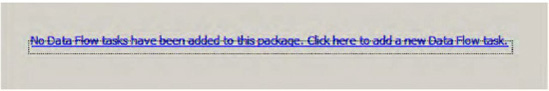
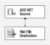
Now double-click on Package.dtsx and open the Data Flow tab. This is where you build the data flow structures you need. You might not have the data flow ready when you run the project first time. Follow the instructions onscreen to enable the Task panel, as shown in Figure 1-19.
Clicking on the link 'No Data Flow tasks have been added to this package. Click here to add a new Data Flow task' (Figure 1-19) would enable the data flow task pane where you can build a data flow by dragging and dropping the tool box items as shown in figure 1.-20. Add an ADO NET Source from the Toolbox to the Data Flow Task panel as shown in Figure 1-20.
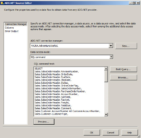
Double-click on the ADO NET Source and configure the Connection Manager (see Figure 1-21). Click the New button and follow the same steps to make the connection.
Under Data access mode, choose SQL command, as shown in Figure 1-21.
Under SQL command text, enter a SQL query or use the Build Query option as shown in Figure 1-22. (Since I had already prepared a script for this, that's what I used. You'll find the SQL script 'salesquery.txt' in the resources available with this book.) Then click on the Preview button to view the data output.
Check the Columns section to make sure the query was successful, then click OK to close the editor window (See Figure 1-23).
From the Data Flow Destinations section on the Toolbox, choose a destination that meets your needs. For this demo, we'll select Flat File Destination.
Drag and drop the Flat File Destination onto the Data Flow Task panel as shown in Figure 1-24. If you see a red circle with a cross mark on the flow controls, hover over the cross mark to see the error.
Connect the green arrow from the ADO NET source to the Flat File Destination.
Double-click on the Flat File Destination, which will open the Editor (Figure 1-25).
Click the New button to open the Flat File Format window, where you can choose among several options. For our demo, select Delimited.
The Flat File Connection Manager Editor window will open next, with options for setting connection manager name and, most importantly, the delimited format, as shown in Figure 1-26. Click OK to continue.
On the next screen, click on Mapping. Choose the Input Column and Destination Columns and then click OK.
The final data flow should look like what's shown in Figure 1-27.
Start debugging by clicking F5, or click Ctrl+F5 to start without debugging.
During the process, you'll see the data flow items change color to yellow.
Once the process completes successfully, the data flow items change to green, as shown in Figure 1-28.
Click the Progress tab to view the progress of the execution of an SSIS package (see Figure 1-29).
Complete the processing of the package by clicking on Package Execution Completed at the bottom of the package window.
Now go to the destination folder and open the file to view the output.
Notice that all the records (28,866) in this case are exported to the file and are comma-separated.
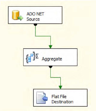
In a more general case, you would probably be using Data Flow Transformations such as Aggregate or Data Conversion. If you did this, the output would then be the aggregation of a chosen input column. You can set the Data Flow Transformations as shown in Figure 1-30.


In many cases, you might actually get a flat file like this as input and want to extract and load it back into your new database or an existing destination database. In that scenario, you'll have to take this file as the input source, identifying the columns based on the delimiter, and load it.
As mentioned before, you may have multiple data sources (such as two sorted datasets) that you want to merge. You can use the merge module and load the sources into one file or dataset, or any other destination, as shown Figure 1-31.
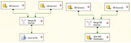
Tip
If you have inputs you need to distribute to multiple destinations, you might want to use Multicast Transformation, which directs every row to each of the destinations.
Now let's see how to move our OLTP tables into an OLAP star schema. As we've chosen tables in the Sales module, let's identify the key tables and data that need to be or can be analyzed. In a nutshell, we need to identify one fact table and other dimension tables first for the Sales Repository (as you see in Figure 1-32).
The idea is to extract data from the OLTP database, clean it a bit, and then load it to the model shown in Figure 1-32. The first step is to create all the tables in the star schema fashion.
Table 1-3 shows the tables you need to create in the AdventureWorksDW database. Once you've created them, move the data in the corresponding tables of the AdventureWorks database to these newly created tables. So your first step is to create these tables with the specified columns, data types, and keys.
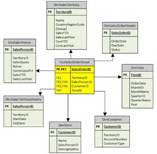
Table 1-3. Tables to create
Table Name | Column Name | Data Type | Key |
|---|---|---|---|
Dim_Customer | CustomerID AccountNumber CustomerType | Int, not null Nvarchar(50), null Nvarchar(3), null | PK |
Dim_DateTime | DateKey FullDate DayNumberOfMonth DayNumberOfYear MonthNumberOfYear MonthName Quarter Year | Int, not null Date, not null Tinyint, not null Tinyint, not null Tinyint, not null Nvarchar(10), not null Tinyint, not null Smallint, not null | PK |
Dim_SalesOrderHeader | SalesOrderHeaderID OrderDate DueDate Status | Int, not null Datetime, null Datetime, null Tinyint, null | PK |
Dim_SalesPerson | SalesPersonID | Int, not null | PK, FK (to SalesPersonID in Dim_SalesTerritoryHistory, Dim_Store tables) |
SalesQuota Bonus CommisionPct SalesYTD SalesLastYear TerritoyID | Money, null Money, null Money, null Money, null Money, null Int, null | FK (to TerritoryID in Dim_SalesTerritory table) | |
Dim_SalesTerritory | TerritoryID Name CountryRegionCode Group SalesYTD SalesLastYear CostYTD CostLastYear | Int, no null Nvarchar(50), null Nvarchar(3), null Nvarchar(50), null Money, null Money, null Money, null Money, null | PK |
Dim_SalesTerritoryHistory | SalesTerritoryHistoryID SalesPersonID TerritoryID StartDate EndDate | Int, not null Int, not null Int, not null Date, null Date, null | PK FK (to SalesPersonID in Dim_SalesPerson table) FK (to TerritoryID in Dim_SalesTerritory table) |
Dim_Store | StoreID CustomerID SalesPersonID | Int, not null Int, not null Int, not null | PK FK (to CustomerID in Dim_Customer table) FK (to SalesPersonID in Dim_SalesPerson table) |
Fact_SalesOrderDetails | SalesOrderID SalesOrderHeaderID DateKey CustomerID TerritoryID | Int, not null Int, not null Int, not null Int, not null Int, not null | PK FK (on SalesOrderHeaderID in Dim_SalesOrderHeader table) FK (to DateKey in Dim_DateTime table) FK (to CustomerID in Dim_Customer table) FK (to TerritoryID in Dim_SalesTerritory table) |
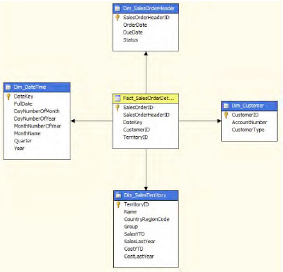
After you build these tables, the final tables and their relations would look pretty much as shown in Figure 1-33.

Notice the Fact_SalesOrderDetails table (fact table) and how it is connected in the star. And the rest of the tables are connected in the dimension model making up the star schema. There are other supporting tables but we'll ignore for a while since they may or may not contribute to the cube.
Note
Make sure the column data types are in sync or at least while extracting the data and loading, alter the data so it matches the column types.
You may be wondering how we came to the design of the tables.
Rule #1 when you create a schema targeting a cube is to identify what you would like to accomplish. In our case, we would like to know about how Sales did with stores, territory, and customers, and across various date and time factors (recollect the cube in Figure 1-6). Based on this, we identify the dimensions as Store, Territory, Date/Time, Customer, Sales Order Header. Each of these dimensions will join to the Facts Table containing sales order details as facts.
As with the SSIS example we did earlier (importing data from a database and exporting to a flat file), we can now directly move the information into these newly generated tables instead of exporting them to the flat files.
One very important and useful data flow transformation is the Script Component, which you can use to programmatically read the tables and columns values from the ADO NET Source (under AdventureWorks database) and write to the appropriate destination tables (under AdventureWorksDW database), using a script. While you do the extraction from the source, you have full control over the data and thus can filter the data, clean it up, and finally load the it into the destination tables, making it a full ETL process. You simply drag and drop the Script Component from the Data Flow Transformations into the Data Flow, as shown in Figure 1-34.

Note
For more information on using the Script Component to create a destination, see the references at msdn.microsoft.com/en-us/library/ms137640.aspx and msdn.microsoft.com/en-us/library/ms135939.aspx.
Tip
Many other operations, including FTP, e-mail, and connecting web services can be accomplished using SSIS. Another good real-time example of when you could use SSIS is when you need to import a text file generated from another system or to import data into a different system. You can run these imports based on schedules.
Now that we've create the tables and transformed the data, let's see how to group these tables in a cube, create dimensions, run an MDX query, and then see for the results.
Microsoft SQL Server Analysis Services (SSAS) is a powerful tool that lets us create and process cubes. Let's now look at how cubes are designed, what the prerequisites are, and how cubes are created, processed, and queried using the MDX query language.
Note
SQL Server 2008 R2 comes with a lot new features. Visit msdn.microsoft.com/en-us/library/bb522628.aspx for more information.
SSAS is used to build end-to-end analysis solutions for enterprise data. Because of its high performance and scalability, SSAS is widely used across organizations to scale their data cubes and tame their data warehouse models. Its simplicity and rich tools give developers the power to perform various drill-down options over the data.
Let's take care of the easy part first. One way to get started with cubes is by using the samples provided with the AdventureWorks database. BIDS sample projects are located at C:program filesmicrosoftsql server100 oolssamplesAdventureWorks 2008 Analysis Services Project. You should have two projects for both the Enterprise and Standard versions.
Open one of the folders based on your server license, then open the AdventureWorks.sln file using BIDS.
Check the Project properties and make sure to set the Deployment Target Server and Database properties.
Build and deploy the solution.
This project contains lots of other resources, including data sources, views, cubes and dimensions. However, these provide information relating to the layout, structure, properties, and so forth of BIDS, and little information about cube structures, and the like.
Once the project is deployed successfully (with no errors), open SSMS. You'll find the cubes from the previous deployment available for access via MDX queries. Later in this chapter you'll learn how to create a simple cube. For now, we'll use the available AdventureWorks cubes.
Executing an Analysis Services MDX query from SSMS involves few steps, as follows:
Run SQL Server Management Studio and connect to the Analysis Services... instance on your server by choosing Analysis Services under Server type.
Click on the New Query button, which launches the MDX Query Editor window.
In the MDX Query Editor window, from the Cube drop-down, select one of the available cubes from the Analysis Services database you're connected to, "AdventureWorks" in this case.
Under the Metadata tab, you can view the various measures and dimensions available for the cube you selected.
Alternatively, you can click on the Analysis Services MDX Query icon at the top to open the query window.
Writing an MDX query is similar to writing a T-SQL query. However, instead of querying from tables, MDX queries from a cube's measures and dimensions.
Enter your MDX query in the query window and execute to view the output, as shown in Figure 1-35.

Ok, so far you've seen the basic cube (using one from the AdventureWorks database) and also how to query from the cube using a simple MDX query. Let's now begin a simple exercise to build a cube from scratch.
Using data from the Sales Repository example we looked at earlier, let's configure a cube now using the Dimension and Fact tables you created manually with the AdventureWorksDW database.
Once you have the data from SSIS in the designated tables (structured earlier in this chapter), you can create a new project under SSAS.
Open BIDS and create a New Project by selecting Analysis Services Project.
Provide a valid project name, such as AW Sales Data Project, a Location, and a Solution Name. Click OK.
A basic project structure is created from the template, as you can see in Figure 1-36.
Create a new data source by right-clicking on Data Sources and selecting New Data Source; this opens the New Data Source Wizard.
Click the New button and choose the various Connection Manager options to create the new Data Connection using the database AdventureWorksDW.
Click Next and choose "Use the service account" for the Impersonation option. You can also choose other options based on how your SQL Server is configured.
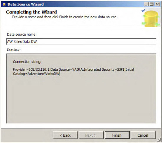
Click Next and provide a valid Data Source Name (AW Sales Data DW in our case) and click Finish, as shown in Figure 1-37.
The next step is to create the data source views, which are important because they provide the necessary tables to create the dimensions. Moreover, a view is the disconnected mode of the database and hence won't have any impact on performance.
Right-click on Data Source Views and choose New Data Source View, which brings up the Data Source View Wizard.
Select an available data source. You should see the AW Sales Data DW source you just created.
Click Next and choose the available tables from the Select Tables and Views window (see Figure 1-38). Select the dimension and fact tables we created earlier and click Next.
To save the data source view, provide a valid name (AW Sales Data View) and click Finish.
Notice that Design View now provides a database diagram showing all the tables selected and the relations between each of them.
Now you can create either a dimension or a cube, but it's always preferable to create dimensions first and then the cube, since the cube needs the dimensions to be ready. Right-click on Dimensions and choose New Dimension, which brings up the Dimension Wizard.
Click Next. On the Select Creation Method screen, choose "Use an existing table" to create the dimension source, then click Next.
On the next screen, choose the available Data source view. For the Main table, select Dim_DateTime and then click Next.
The next screen displays the available attributes and types (see Figure 1-39). Notice the attribute types that are labelled "Regular." By default, only the primary keys of the tables are selected in the attributes for each dimension. You need to manually select the other attributes. This step is important since these are the values you query in MDX along with the available measures.
Choose the attributes Month Name, Quarter, and Year in our sample and change the attribute types to Month, Quarter, and Year, respectively, as shown in Figure 1-39. Click Next.
Provide a logical name for the dimension (Dim_Date in our case) and click on Finish. This creates the Dim_Date.dim dimension in the Dimensions folder in your project.
In Solutions Explorer, right-click on the Cubes folder and choose New Cube to bring up the Cube Wizard welcome screen. Click Next.
On the Select Creation Method screen, choose "Use existing tables" and then click Next.
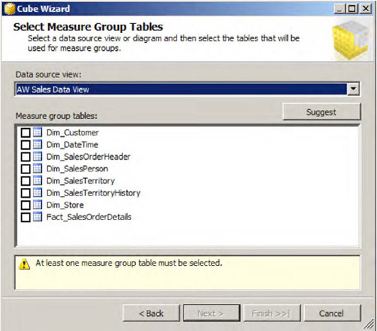
From the available Measure group tables, select the fact table or click the Suggest button (see Figure 1-40.
If you choose Suggest, the wizard will select the available measure group tables. You can choose your own Measure Group tables in the other case. Click Next to continue.
The Select Measures screen displays the available measures, from which you can either select all or just what you need. Leave the default to select all and click Next to continue.
Now you can choose to Select Existing Dimensions from any available. For now, you can leave the default—the existing dimension. Click Next to continue.
The Select New Dimensions screen gives us the option to choose new dimensions that the wizard identifies from the data source selected. If you have already chosen a dimension in the previous step, ignore that dimension or just click Next to continue. If you have previously created a dimension and also selected the same one that's listed here, the wizard would create another dimension with a different name. Click Next.
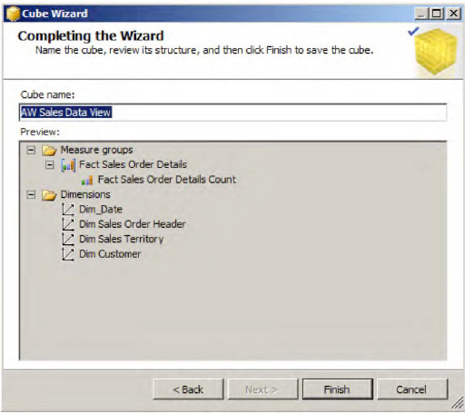
Provide a valid cube name, AW Sales Data View, as shown in Figure 1-41. Notice that Preview displays all the measures and dimensions chosen for this cube. Click Finish to complete the step.
The cube structure will now be displayed in the form of star, with the fact table in the center (yellow header) and the dimensions around it (blue header), as shown in Figure 1-42.
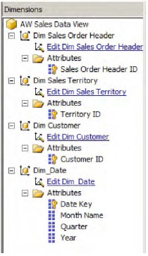
In the Dimensions window (usually found in the bottom left corner), expand each of the dimensions and notice that the attributes are just the primary key columns of the table (see Figure 1-43). You need all the attributes or at least the important columns you wish to run analysis on.
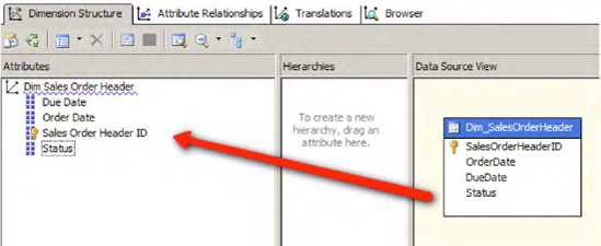
From the Dimensions folder in Solution Explorer, double-click each of the dimensions to open the Dimension Structure window (Figure 1-44).
Choose the Dimension columns from the Data Source View pane and drop them on the Attributes pane as shown in Figure 1-44.
Repeat the same steps for the rest of the dimensions and click Save All. Refresh the window and notice that all columns now appear under attributes and have been added to the Dimensions.
To add hierarchies, drag and drop the attribute(s) from the Attributes pane to the Hierarchies pane. Repeat the step for all of the dimensions. When you're done, go back to the Cube Structure window.
On the left hand in the Measures pane, you now have only one measure—Fact Sales Order Details Count. To create more measures, simply right-click on the Measures window and choose New Measure.
From the New Measure dialog box, select the option "Show all columns".
For the Usage option, select Sum as the aggregation function. Then choose Dim_SalesTerritory as the Source Table and SalesYTD as Source Column, and click OK. What this does is provide a new measure, Sales YTD, by summing the values from a given territory against the available dimensions.
All is well at this time. Our final window looks something like what's shown in Figure 1-45.
Now right-click on the project properties and check the deployment options. Leaving the options as is would deploy the project to the local SQL Server. Right-click again on the project properties and select Deploy.
This step builds and deploys the project to the target server. You can view the deployment status and output in the deployment progress window.
If the deployment is successful, you'll see a "Deployment Completed Successfully" message at the bottom of the progress window, as shown in Figure 1-46.
On the Connect to Server dialog box (Figure 1-47), choose Analysis Services as the Server type, provide a Server name and credentials if applicable, and click on Connect.
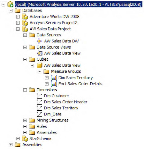
Object Explorer displays the available databases. You'll find the AW Sales Data Project you created earlier in BIDS and deployed locally. Expand the options and notice various entities available under the Data Sources, Data Source Views, Cubes and Dimensions (see Figure 1-48).
Click on the MDX Query icon on the toolbar to open the query window and the cube window. Make sure the appropriate data source is selected at the top.
The cube will display the available Measures and Dimensions, as shown in Figure 1-49.
In the query window, type the MDX query to retrieve the values from the cube. In our case, to get the Sum of Sales YTD in the Sales Territory Measure, the query should look like the one in Figure 1-49.
Execute and parse the query to view the output in the results window.


Now that you know the concepts, let's see some of the important factors to keep in mind while planning for a migration. First, you need to be completely aware of why you need to migrate to an OLAP database from an OLTP database. If you are not clear, it's a good idea to go back to the section "Why do I need to migrate to OLAP?" and make a checklist (review as well the need for a staging section).
Make sure that there is no mismatch in column names on both ends. Well, this is not a requirement. Most of the time, you don't have same columns. In such cases, maintain metadata for the mapping. ETL tools (in this case SSIS) support different column names.
While mapping columns between source and destination, there is a good possibility that the data types of the columns might not match. You need to ensure type conversion is taken care during transformation.
With OLAP, the idea is to restrict the number of columns and tables and denormalize as much as possible. So, it's a good idea to remove unwanted columns.
You already know that data can be migrated from different data sources—such as databases, flat files, XML, Excel, and so forth—to a single OLAP system of your choice. OLAP tools provide the necessary framework to accomplish this.
Migrating data from OLTP system to OLAP is as good as copying and pasting your enterprise database. Clean up the data either during staging or during the transformation process to avoid unwanted data.
What you have in many tables in your OLTP database might be aggregated into a single table or even one column.
Move to more sophisticated and structured cubes. Review decision support systems and data mining systems and choose your model accordingly.
Use the features of ETL tools efficiently for migration.
We won't actually be using SQL Server 2008 R2 Parallel Data Warehouse in our explorations here, but it's worth mentioning as it can provide a robust foundation for business intelligence.
What is the new parallel data warehouse from SQL Server 2008 R2? It's a combination of hardware and software that uses a massively parallel architecture and industry-standard hardware to enormously increase performance and scalability when analyzing data. And it's not just for SQL Server databases but also extends the power for Oracle databases and others. Key features and capabilities include:
Scalability supporting hundreds of terabytes of data
Low cost
Tight integration with existing SQL Server 2008 data warehouses using hub-and-spoke architecture
High performance
ROI improvements using SQL Server BI Tools.
However, as noted above, it's a software/hardware combination that requires SQL Server 2008 R2 to run on specific hardware to provide the advantages and capabilities. Business need to have the OEM hardware/software packages (provided by Bull, Dell, EMC, HP, and IBM) to get the optimized scalability and performance. For more details on SQL Parallel Data warehouse, please visit microsoft.com/sqlserver/2008/en/us/parallel-data-warehouse.aspx
What do you have so far?
Microsoft Office SharePoint Server (MOSS) 2007 has decent capabilities relating to BI integration. Major components include Excel Services, Reporting Services and Dashboards.
SSIS components can extract information from various data sources, and load it into Excel and it can be published back into SharePoint. This enables possibilities for seamless end-to-end integration and collaboration using the portals.
Business applications use powerful out of the box web parts that can display their KPIs.
The BDC (Business Data Catalog) provides a mechanism for integrating external data sources into the system.
Note
By now you have some familiarity with business intelligence and some of the components of OLAP. For more information, please visit microsoft.com/casestudies/.
SharePoint 2010 adds significantly more BI functionality. In the next chapters we will cover each of SharePoint 2010's BI components in depth. Here's a preview.
Remember the single sign-on (SSO) functionality in MOSS 2007? SharePoint 2010 introduces Secure Store Service (SSS) as its next-generation SSO. This claims-aware (that is, using claims-based authentication) service is part of the Foundation Server and it enables mechanisms by which you store credentials for each application by ID, and reuse the credentials to gain access to external data sources. Visio Services, PerformancePoint Services, and Excel services work in conjunction with Secure Store Services. We will examine SSS in Chapter 2.
Note
For more information on Secure Store Service, please see Chapter 12 of Building Solutions with SharePoint 2010 by Sahil Malik (Apress, 2010).
What if Visio diagrams came alive? Can they be powered by data in real time? The answer is yes! Visio Services is now available as part of SharePoint 2010 Enterprise edition, allowing you to connect real-time data and update your Visio diagrams on the fly. Share and view published Visio diagrams using the Visio Web Access Web Part, which provides the functionality to integrate Visio diagrams into the SharePoint platform. With a basic knowledge of JavaScript and the client object model, you can create compelling, rich, interactive UIs. Learn more about Visio Services in Chapter 2.
A lot of new functionality has been added to Reporting Services in SharePoint 2010. New features include support for claims-based authentication and user tokens, deployment utilities, support for multiple languages, and connectivity with list and document libraries.
Because report-authoring tools are an integral part of SQL Server Tools, they are integrated in SharePoint so that generating and customizing reports has been easy in a SharePoint Server (as well as MOSS 2007) environment.
Out-of-the-box Reporting Services web parts take care of other needs by providing a platform to load reports designed using Report Builder. Learn more about Reporting Services in Chapter 3.
With SharePoint 2010, PerformancePoint Services is now available as an integrated part of the SharePoint Server Enterprise license. You can now consume context-driven data, build dashboards with the help of the built-in Dashboard Designer, and take advantage of KPIs, and scorecards. Data from various sources can be integrated using SSIS, loaded using SSAS, and finally published into SharePoint. Support for SharePoint lists and Excel Services are additional benefits. The RIA-enabled Decomposition Tree is a powerful new visualization report type that lets you drill down into to multidimensional data. Learn more about PerformancePoint Services in Chapter 4.
Excel Services is also available now as part of SharePoint Server Enterprise licensing, and now support multiple data sources aggregation in a single Excel workbook. Excel Services allows these workbooks to be accessed as read-only parameterized reports via the thin web client. You can choose to expose the entire workbook or only portions of the workbook, such as a specific chart or a specific pivot table. Content in Excel can be accessed though various methods, such as REST services, Web Services, publishing to the SharePoint environment, and using JavaScript.
With the addition of PowerPivot to Excel 2010 and its in-memory data store capabilities, it's now possible to connect to the OLAP data sources that give users the flexibility to analyze their data. Learn more about Excel Services and PowerPivot in Chapter 5.
Business Connectivity Services (BCS) is a part of SharePoint 2010 Composites, prebuilt components you can use to create custom business solutions. BCS is the next version of Moss's well-known Business Data Catalog. BCS is now bi-directional (in that it can both display business data and, with appropriate permissions, update it), and it is much easier now to connect with various other systems. Tools such as SharePoint Designer and Visual Studio provide the functionality that lets you connect with external data sources such as SQL Server, WCF services, and .NET connector assemblies. Visual Studio and custom code make it possible to address almost any problem. While Business Data Connectivity services, External Data columns and External lists are available in the Foundation Server, data search, profile pages, and Secure Store belong to Standard version, and the rest of the external data Web Parts, and Office Client Integration reside under Enterprise Client Access License (CAL). Learn more about BCS in Chapter 6.
This chapter introduced you to
Why you need business intelligence.
The various elements of BI, as shown in Figure 1-50.
Data warehouse components, OLAP, and cubes.
Querying from OLAP using MDX.
Understanding SQL Server tools for BI, including SSIS and SSAS.

Note
By now you have some familiarity with business intelligence and some of the components of OLAP. For more information on busines intelligence, please visit http://www.microsoft.com/casestudies/