7.1 Introduction

In Chapter 6, we have considered large sample statistical estimation and hypotheses testing techniques which depend on the central limit theorem to justify normality of the estimators and the test statistics. They apply when the samples are large (n ≥ 30).

Situations arise where large sampling is not possible. Consider, e.g., populations such as synthetic diamonds, satellites, aeroplanes, super computers and nuclear reactors which involve heavy expenditure. In such cases, the size of the sample is small (n < 30) and we have to consider statistical techniques that are suitable for them.

7.2 Test for One Mean (Small Sample)

7.2.1 Student's t-Distribution

While discussing sampling distribution, we noted the following points:

1. When the original sampled population is normal, and both have normal distributions for any sample size n.
2. When the original sampled population is not normal, and both have ­approximately normal distributions, if the sample size n is large.

But when the sample size n is small, the statistic does not have normal distributions. In such a case, there are two ways to proceed:

1. We use an empirical approach. We draw ­repeated samples and compute for each sample. The ­relative frequency distribution that we construct using these values will approximate the shape and locations of the sampling distribution.
2. We use a mathematical approach to derive the actual density function or curve that describes the sampling distribution.

The second approach was used by an English statistician W. S. Gosset in 1908. He derived a complicated formula for the density function of for random samples of size n from a normal population. He published his results under the pen name ‘Student’ and hence the statistic has been known as Student's t-distribution. It has the following characteristics:

1. It is mound shaped and symmetric about t = 0 just like Z.
2. It is more variable than z. It has heavier tails. That is the t-curve approaches the horizontal axis more slowly when compared with the normal curve. This is due to the fact that t-statistic involves two random quantities and s whereas the Z-statistic involves only the sample mean (Figure 7.1).
   

   Figure 7.1 Standard normal Z and t-distributions.

3. The shape of the t-distribution depends on the sample size n. As n becomes larger, the variability of t decreases because the estimate of s of σ is based on more and more information. Consequently, when n is infinitely large, the t and Z distributions are identical.

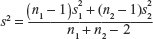
   The sample variance s² is given by the ­formula

   

   or by

   

   where is the sum of the squares of the individual sum of the squares of the individual measurements and is the square of the sum of the individual measurements.

The divisor (n − 1) in the formula is called the number of degrees of freedom (dof) associated with s². It determines the shape of the t-distribution. The term ‘degrees of freedom’ refers to the number of independent deviations in s² that are available for estimating σ². The dof may be ­different for different applications and may specify the correct t-distribution to be used.

For calculating critical values or p-values for the t-statistic, the table of probabilities for the standard normal Z-distribution is not useful. Instead, we have to use the t-distribution table.

For a t-distribution with 5 dof, the value of t that has area 0.05 to its right is found in row 5 in the column t_0.05. For this particular t-distribution, the area to the right of t = 2.015 is 0.05. Only 5% of all values of the t-statistic will exceed this value.

Example 7.1

Suppose that we have a sample of size n = 10 from a normal distribution. Find the value of t such that only 1% of all values of t will be smaller than this.

Solution The dof that give us the correct ­t-distribution are n − 1 = 10 − 1 = 9. The ­required t-value must be in the lower portion of the t-distribution with area = 0.01, i.e. 1%, to its left (Figure 7.2). Since the t-distribution is ­symmetric w.r.t. 0, this value is the negative of the value on the right-hand side with area 0.01 to its right, i.e. − t_0.1 = −2.821.

Assumptions Relating to Student's ­t-Distribution The critical values of t permit us to make reliable inferences only if we follow all the rules. This implies that the sample must meet the following requirements specified by the t-distribution:

1. The sample must be randomly selected.
2. The population from which sampling is done must be normally distributed.

7.2.2 Small Sample Inferences Concerning a Population Mean

We have considered large sample inferences in Section 7.2.1. As with large sample inference, small sample inference may involve either estimation or hypothesis testing. Instead of Z-statistic and normal distribution, we will use a different sample statistic, namely, and a different sampling distribution, namely, the Student's t-distribution with (n − 1) dof.

Small Sample Hypothesis Test for m

1. Null hypothesis (NH) H₀: μ = μ₀
2. Alternative hypothesis (AH) H₁: μ < μ₀
   1. (a) One-tailed test: H₁: μ > μ₀ or H₁: μ < μ₀
   2. (b) Two-tailed test: H₁: μ ≠ μ₀
3. Test Statistic:
4. 4. Rejection Region: Reject H₀ when
   1. One-tailed test: t > t_α or t < − t_α when the AH is H₁: μ < μ₀ or p value < α
   2. Two-tailed test: t > t_{α /2} or t < − t_{α /2}

      The critical values of t, t_α and t_{α /2} based on (n − 1) dof are shown in Figure 7.3. These values are found in the t-distribution table.

Figure 7.3 Critical values of t, t_α and t_{α /2} based on (n − 1) dof.

Small Sample (1 − α) 100% Confidence ­Interval for μ It is

where is the estimated standard error of It is called the standard error of the mean.

Two Ways to Conduct a Test of Hypothesis They are as follows:

1. Critical Value Approach Based on the ­critical value of the sampling distribution of the test ­statistic, we set up rejection region. If the test statistic falls within the rejection region we can reject H₀.
2. p-Value Approach Based on the observed value of the test statistic, calculate the p-­value. If it is smaller than the LOS α, we can reject H₀.

Note Example 7.2 uses the first approach and Example 7.3 uses the second approach.

Example 7.2

A new process of producing synthetic diamonds can be operated at a profitable level only if the average weight of the diamonds is greater than 0.5 carat. To test the profitability of the process, 6 diamonds are produced with weights 0.45, 0.60, 0.52, 0.49, 0.58 and 0.54 carat respectively. Do the 6 measurements present sufficient evidence to indicate that the average weight of the diamonds produced by the process is in excess of 0.5 carat?

Solution The mean of the population of the diamonds produced by the new process is μ = 0.5.

Mean of the weights of the six diamonds is

= (0.45 − 0.53)² + (0.60 − 0.53)² + (0.52 − 0.53)² + (0.49 − 0.53)² + (0.58 − 0.53)² + (0.54 − 0.53)²

= (− 0.08)² + (0.07)² + (−0.01)² + (− 0.04)² + (0.05)² + (0.01)²

= 0.0064 + 0.0049 + 0.0001 + 0.0016 + 0.0025 + 0.0001

= 0.0156

Sample size n = 6

Sample variance

Sample standard deviation

We now carry out the formal test of hypothesis in steps as follows:

1. NH H₀: μ = 0.5
2. AH H₁: μ > 0.5
3. Test Statistic:

   The test statistic provides evidence for either rejecting or accepting H₀ depending on how far from the centre of the t-distribution does the test statistic lie.

4. Rejection Region: Let us choose a 5% LOS, i.e. α = 0.05. The right-side tail rejection ­region is found using the critical values of t from the t-distribution table.

   Number of dof = n − 1 = 6 − 1 = 5

   So, we can reject H₀ if t > t_0.05 = 2.015, as shown in Figure 7.4.

   

   Figure 7.4 Rejection region for example 7.2.

5. Conclusion: Here the calculated value of test statistic is t = 1.3155. It does not fall within the rejection region. Therefore, we cannot reject H₀. Hence the data do not give sufficient evidence to indicate that the mean diamond weight exceeds 0.5 carat.
6. 6. Remarks: The conclusion to accept H₀ requires the difficult calculation of β. This is the case of Type II error. To avoid this, we choose not to reject H₀. Towards this end, we consider a 95% lower one-sided confidence bound for μ as follows:

   

   = 0.53 − 0.04595 = 0.484

Thus, a 95% lower bound for μ is μ > 0.484. The range of possible values includes mean diamond weights both smaller and greater than 0.5. This confirms the failure of our test to show that μ exceeds 0.5.

Example 7.3

Labels on one-gallon cans of paint indicate the ­drying time and the area that can be covered in one coat. A manufacture of paints claims that the brand of paint they manufacture will cover 420 sq. ft per 1 gallon. To test this, a random sample of 10 one-gallon cans of paints was tested. The actual areas painted in sq. ft are 362, 356, 413, 422, 372, 416, 376, 434, 388 and 421.

1. Do the data present sufficient evidence to indicate that the average differs from 425 sq. ft?
2. Find the p-value for the test and use it to evaluate the statistical significance of the results.

Solution

1. First we calculate the mean of the ­sample

   [362 + 356 + 413 + 422 + 372 + 416 + 376 + 434 + 388 + 421] = 396

   Next, we find the sample variance

   s² =

   [(362 − 396)² + (356 − 396)² + (413 − 396)² + (422 − 396)² + (372 − 396)²

   + (416 − 396)² + (376 − 396)² + (434 − 396)² + (388 − 396)² + (421 − 396)²]

   [(− 34)² + (− 40)² + (17)² + (26)² + (− 24)² + (20)² + (− 20)² + (38)² + (− 8)² + (25)²]

   = 803.3333

   Now, the standard deviation is

   

   We calculate the test statistic

   

   The p-value for the test is the probability of observing a value of the t-statistic as contradictory to NH. For the above set of data, we have obtained t = −2.678. This is a two-tailed test. The p-value is the probability that either t ≤ − 2.678 or t ≥ 2.678.

   From the t-distribution tables, we observe that it gives values of t corresponding to right-side tail areas. Since in the present case dof = n − 1 = 9, we read the areas ‘α’ in row 9 corresponding to the values of t:

   

   The five critical values for various tail areas are also shown in Figure 7.5.

   

   Figure 7.5 p-value for example 7.3.

   The value t = 2.678 falls between 2.262 and 2.821 which correspond to t_0.025 and t_0.010 respectively.

   This area represents only half of the p-value. We have 0.01 < (p-value) < 0.025 ⇔ 0.02 < p-value < 0.05, so reject H₀ at the 5% level but not at the 2% or 1% level. Therefore, the p-value is less than 0.1.

   For this test of hypothesis, H₀ is rejected at the 5% LOS. There is sufficient evidence to indicate that the average coverage differs from 420 sq. ft.

2. Limits for the actual average coverage A 95% confidence interval gives the limits for μ as

   

   = (375.73, 416.27)

   We can estimate that the average coverage of area by one gallon of paint lies in the interval (375.73, 416.27). If we increase the size of the sample, a shorter interval can be obtained.

   Observe that the upper limit of the interval 416.27 is close to 420 sq. ft, the coverage claimed on the label. The observed value of t is −2.678 which is slightly greater than the left critical value of t_0.05 = −2.821, making the p-value slightly more than 0.05.

7.3 Test for Two Means

7.3.1 Small Sample Test Concerning Difference ­Between Two Means

Let n₁ and n₂ be the two sides of two samples, which are small (i.e. n₁ and n₂ < 30). Suppose that these samples are drawn from two normal populations with population variances and unknown but equal (i.e. σ₁ = σ₂ = σ ). Then the pooling variance σ² is given by

where and are the mean and variance of two samples of sizes n₁ and n₂ respectively. In a test concerning the difference between the means for small samples, the t-test statistic is given by

with (n₁ + n₂ − 2) dof. This test is also known as two-sample pooled t-test. The above formula can be rewritten as

with (n₁ + n₂ − 2) dof.

Test of Hypothesis Concerning the Difference between Two Means Based on Independent Random Samples

1. NH H₀: μ₁ − μ₂ = δ H₀:μ₁ − μ₂ = δ where δ is some specified difference that you wish to test. In many tests it may be assumed that there is no difference between μ₁ and μ₂ so that δ = 0.
2. AH
   1. One-tailed test: H₁: μ₁ − μ₂ > δ or H₁: μ₁ − μ₂ < δ
   2. Two-tailed test: H₁: μ₁ − μ₂ ≠ δ
3. Test Statistic:

   

   where

   

4. Rejection Region: Reject H₀ when
   1. One-tailed test: t > t_α or t < − t_α when the AH is H₁: μ₁ − μ₂ < δ or when p value < α
   2. Two-tailed test: t > t_{α /2} or t < − t_{α /2}

   The critical values of t, t_α and t_{α /2} are based on (n₁ + n₂ − 2) dof.

Small Sample (1 − α) 100% Confidence Interval for ( μ₁ − μ₂) Based on Independent Random Samples

where s² is the pooled estimate of σ ².

Example 7.4

In a manufacturing company, a one-month training programme is conducted to each employee. A new training programme has been developed. To test the new programme, 2 groups of 9 employees each were assigned a job, the first group trained under the old system and the second trained under the new programme. Their performance timings in minutes are recorded as follows:

Do the job execution times present sufficient evidence to indicate that the mean time is less for the new training programme?

Solution Let μ₁ and μ₂ be the mean time to execute the job after the old and new training programmers respectively. Then, as we would like to gather evidence to support the theory that μ₁ > μ₂, we test the following:

1. NH H₀: μ₁ = μ₂ or H₀: μ₁ − μ₂ = 0
2. AH H₁: μ₁ > μ₂ or H₁: μ₁ − μ₂ > 0
3. Test Statistic: In order to conduct the t-test for these two independent samples, we ­assume that the sampled populations are both normal and have the same variance σ².

   We have

   

   

   

   

   

   [(− 4)² + 3² + 1² + (− 5)² + 7² + (− 1)² + (− 3)² + (− 2)² + 4²]

   (16 + 9 + 1 + 25 + 49 + 1 + 9 + 4 + 16)

   

   

   [(+ 3)² + 2² + (− 5)² + 5² + 0 + (− 3)² + (− 4)² + (− 2)² + 4²]

   (9 + 4 + 25 + 25 + 0 + 9 + 16 + 4 + 16)

   

   Next, we have the standard deviations of the two samples as

   

   

   There is no significant variation between these figures and we may assume that the two distributions are of the same shape.

   We now calculate the pooled estimate of the common variance as

   

   

   We then calculate the test statistic t given by

   

   Here the number of dof is n₁ + n₂ − 2 = 9 + 9 − 2 = 16.

4. Rejection region: The alternative hypothesis H₁: μ₁ > μ₂ or H₁: μ₁ − μ₂ > 0 ­implies that we have to use a one-tailed test on the right-side tail of the t-distribution with 16 dof. The ­appropriate critical value for a ­rejection region with α = 0.05 from the Student's t-distribution table can be found and H₀ will be rejected if t > 1.746. The ­observed value of test ­statistic t is 2.2. Comparing this with the ­critical value t_0.05 = 1746 we can reject H₀. There is ­sufficient evidence to indicate that the new ­training programme is superior at the 5% LOS (Figure 7.6).
   

   Figure 7.6 Rejection region for example 7.4.

5. 5. Conclusion: Since the observed test statistic value t = 2.2 is greater than the critical value t_0.025 = 2.120, we can conclude that the new training programme excels at the 2.5% LOS.

Example 7.5

Find the p-value that would be reported for the statistical test of Example 7.4.

Solution The observed value of t for this single-tailed test is t = 2.2 for a t-statistic with 16 dof. The observed value of t = 2.2 lies between t_0.025 = 2.120 and t_0.01 = 2.583 and the tail area to the right of t = 2.2 is between 0.01 and 0.025. The p-value for this test would be reported as 0.01 < p-value < 0.025.

Since the p-value is less than 0.025, most researches would report the results as significant.

7.3.2 Paired Sample t-Test

Let μ₁ and μ₂ be the unknown means of two samples of the same size n drawn from two normal ­distributions. We would like to test NH that the means are equal μ₁ = μ₂ against the AH μ₁ = μ₂ (say). The variances need not be known but are assumed to be equal.

Suppose each value of the first sample corresponds precisely to one value of the other because corresponding values result from the same person, animal or thing (paired comparison). For example, two measurements of the same thing by two different methods or two measurements from the two eyes of the same person or animal. More generally, they may result from pairs of similar individuals or things, e.g. identical twins and pairs of used front tyres from the same car.

In such cases, we have to form the differences of corresponding values and test the hypothesis that the population corresponding to the differences has mean zero. If the two samples are not independent, we cannot use the previous method.

Paired t-test is applied for n paired observations, which are dependent, by taking the signed differences d_i (i = 1, 2, …, n) of paired data. To test whether the differences d form a random sample is from a normal population with μ₀ = d₀, use large sample test, otherwise use sample t-test if the sample is small (n < 30). The one-sample test in this case is known as paired sample t-test or matched pairs t-test or simply the paired t-test.

The test statistic for the paired t-test is

with v = n − 1 dof

where

is the mean

is the variance and the positive square root is the standard deviation of the differences d_i (i = 1, 2, …, n)

Example 7.6

The following are the average weekly losses of worker-hours due to accidents in 10 industrial units before and after introduction of certain safety measures.

Use 0.05 LOS to test whether the safety measures are effective.

Solution In this problem, the independent sample test is not applicable because the data in the first row and that in the second row are correlated. There is thus obvious pairing of the two sets of ­observations. We apply the paired t-test to the data following the usual steps:

1. NH H₀: μ₁ − μ₂ = μ_d = 0
2. AH H₁: μ₁ − μ₂ = μ_d > 0
3. LOS a = 0.05
4. Criterion: The value of t_0.05 = 1.833 for n − 1 = 10 − 1 = 9 dof.
5. Rejection region: Reject H₀ if t > 1.833
6. Calculation: d_i = (7, 16, 13, −2, 3, 7, 8, −10, 8, 0)

   Mean of differences

   

   Variance [2² + 11² + 8² + (-7)² + (-2)² + 2² + 3² + (-15)² + 3² + (-5)^2]

   (4 + 121 + 64 + 49 + 4 + 4 + 9 + 225)

   

   Standard deviation

7. Test Statistic:

   

8. Conclusion: The observed t-statistic value is t = 2.0922. This figure exceeds the critical value of t, viz. t_0.05 = 1.833 at v = n − 1 = 10 − 1 = 9 dof. Hence, we conclude that the industrial safety measures adopted are effective and the evidence is strong to this effect.

   9. p-Value: The observed t-statistic value viz. t = 2.09 lies between t_0.05 = 1.833 and t_0.025 = 2.262 at 9 dof and the tail area to the right of t = 2.09 is between 0.025 and 0.05. The p-value for this test would be reported as 0.025 < p-value < 0.05. Since the p-value is less than 0.05, most researches would report the results as significant.

Example 7.7

In Example 7.6, find a 90% confidence interval for the mean improvement in lost worker-hours.

Solution Here n = 10, mean of the differences Also, the standard deviation s_d = 7.56. Since t _0.05 = 1.833 at 9 dof, the 90% confidence interval for μ_d, the mean improvement, is

0.62 < μ_d < 9.38

We conclude that 90% confidence interval for the mean improvement in lost worker hours per week is lost, on an average, after the implementation of the safety measures in the industrial unit.

7.4 Test of Hypothesis

7.4.1 Test of Hypothesis: One Proportion (Small Sample)

Tests of hypothesis concerning proportions are required in many areas.

Examples

1. A politician is interested in knowing what fraction of the voters will favour him in the next ­election.
2. All manufacturing companies are concerned about the proportion of defective items while ­marketing.
3. A gambler wishes to know what proportion of outcomes would be favourable to him.Consider the problem of testing the hypothesis that the proportion of success in a binomial experiment is equal to a given value. The steps for testing an NH about a proportion against various alternatives using the binomial probabilities are the following:
   1. NH H₀: p = p₀
   2. AH H₁: p < p₀
   1. One-tailed test: H₁: p > p₀ or H₁: p < p₀
   2. Two-tailed test: H₁: p ≠ p₀
4. Choose an LOS
5. Test Statistic: Binomial variable x with p = p₀
6. Computations: Find x, the number of success and compute the appropriate ­p-value
7. Conclusion: Draw appropriate conclusions based on the p-value

Example 7.8

A builder claims that heat pumps are installed in 70% of all homes being constructed today. Would you agree with this claim if a random survey of new homes shows that 8 out of 15 had heat pumps installed? Use a 0.10 LOS.

Solution

1. NH H₀: p = 0.7
2. AH H₁: p ≠ 0.7
3. LOS a = 0.10
4. Test statistic: Binomial variable x with p = 0.7 and n = 15
5. Computations: x = 8 and np₀ = 15(0.7) = 10.5. From the table of binomial probability sums, we find that the computed value of p is

   

6. 6. Conclusion: Do not reject H₀. We conclude that there is insufficient reason to doubt the builder's claim.

7.4.2 Test of Hypothesis: One Proportion (Large Sample)

For large samples, normal curve approximation with parameters μ = np₀ and σ² = np₀q₀ is usually preferred for large n. This gives accurate results as long as p₀ is not extremely close to 0 or 1. For using normal approximation, the Z-value for testing p = p₀ is given by

which is a value of the standard normal variable Z. Hence, for a two-tailed test at the LOS α, the critical region is Z < − Z_α/2 and Z > Z_α/2. For one-sided alternative p < p₀, the critical region is Z < − Z_α and for the alternative p > p₀, the critical region is Z > Z_α.

Example 7.9

A commonly prescribed drug for relieving nervous tension is believed to be only 60% effective. Experimental results with a new drug administered to a random sample of 100 adults who had been suffering from nervous tension show that 70 received relief. Is this sufficient evidence to conclude that the new drug is better? Use a 0.05 LOS.

Solution

1. NH H₀: p = 0.6
2. AH H₀: p > 0.6
3. LOS a = 0.05
4. Critical region Z > 1.645
5. Computations: Here x = 70 and n = 100

   np₀ = 100 × 0.6 = 60

   

   p = P (Z > 2.04) < 0.025

6. Conclusion: Reject H₀. We conclude that the new drug is superior.

7.4.3 Test of Hypothesis: Two Proportions

Let A and B be two distinct populations and suppose each member of these populations belongs to two mutually exclusive classes depending on whether it possesses an attribute C (success) or not (failure).

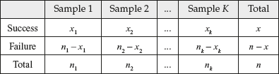
Let x₁ and x₂ be the number of items possessing attribute C in random samples of sizes x₁ and x₂ drawn from the two population A and B respectively (Table 7.1).

Table 7.1 Success and failure in random samples of sizes n₁ and n₂ from two populations A and B.

Then and are the sample proportions.

Let p₁ and p₂ be the population proportions of A and B respectively. To determine whether the proportion of items having attribute C (success) is same in both the population tests, the steps are as follows:

1. NH H₀: p₁ = p₂ or p₁ − p₂ = 0
2. Against AH H₁: p₁ < p₂
   1. One-tailed test: H₁: p₁ > p₂ or H₁: p₁ < p₂
   2. Two-tailed test: H₁: p₁ ≠ p₂

For large samples when n₁ and n₂ ≥ 30, p₁ and p₂ are asymptotically normally distributed and hence the sampling distribution of differences in proportions (p₁ − p₂) will be approximately normally distributed with mean and standard deviation is given by

Here, an unbiased pooled estimate of the population proportion p^ is

obtained by pooling together the data from both the samples.

∴ Z-statistic for testing p₁ = p₂ is given by

Using the critical points of the standard normal curve, the critical regions are determined depending on the appropriate AH.

Example 7.10

If 120 out of 200 patients suffering from a certain disease are cured by allopathy and 240 out of 500 patients are cured by homeopathy, is there reason enough to believe that allopathy is ^­better than homeopathy in curing the disease? Use α = 0.05 LOS.

Solution Let p₁ and p₂ be the proportions of patients cured by allopathy and homeopathy ­respectively.

1. NH H₀: p₁ = p₂

   There is no difference between allopathy and homeopathy.

2. AH H₁: p₁ > p₂

   Allopathy is better than homeopathy.

3. LOS α = 0.05

   Reject H₀ if critical region Z > 1.645

4. Computations: By a right-side one-tailed test,

   

   

   Pooled proportion

   

   

   

   p = p (Z > 2.9) = 0.0019

5. Conclusion: Reject H₀ and agree that the proportion of patients following allopathy is higher than the proportion following homeopathy, i.e. allopathy is better than homeopathy in curing particular disease.

7.4.4 Test of Hypothesis for Several Proportions

Consider K as the binomial populations with parameters p₁, p₂, …, p_k to test whether the population proportions of these K populations are all equal. Consider the following:

1. NH H₀: p₁ = p₂ = … = p_k
2. Against AH H₁: p_i ≠ p_j for some i, j
3. Computations: Let us draw K independent random samples of sizes n₁, n₂, …, n_k, one from each of the K populations. Let n₁, n₂, …, n_k denote the number of items possessing the attribute (success) Table 7.2.

   Here n denotes the total number of trails and x denotes the total number of successes for all the samples put together. The expected cell frequencies e_ij are calculated by

   Table 7.2 Success and failures of all samples.

   

   

   

   ⋮

4. Test Statistic: Difference among the proportions is given by

   

   where o_ij are the observed cell frequencies and e_ij are the expected cell frequencies.

5. Conclusion: Reject H₀ if

Example 7.11

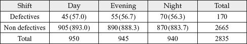
In a shop study, a set of data was collected to determine whether or not the proportion of defectives produced by workers was the same for the day, evening or night shift worked (Table 7.3).

Use a 0.025 LOS to determine if the proportion of defectives is the same for all three shifts.

Solution Let p₁, p₂ and p₃ represent the true proportions of defectives for the day, evening and night shifts respectively.

1. NH H₀: p₁ = p₂ = p₃
2. AH H₁: p₁, p₂ and p₃ are not all equal.
3. LOS α = 0.025
4. Critical Region: χ² > 7.378 for v = 2 dof
5. Computations: Corresponding to the observed frequencies o₁ = 45 and o₂ = 55, we find the following expected frequencies:

   

   

   All other expected frequencies are found by subtraction and are displayed in Table 7.4.

   Table 7.4 Observed and expected frequencies.

   

   

   

   

   and

   p = 0.04

6. 6. Conclusion: We do not reject H₀ at α = 0.025. With the above p-value computed, it would ­certainly be improper to conclude that the proportion of defectives produced is the same for all shifts.

7.5 Analysis of r × c Tables (Contingency Tables)

A classification in which attributes are divided into more than two classes is called a manifold classification. Let an attribute A be divided into r classes A₁, A₂, …, A_r and another attribute B be divided into c classes B₁, B₂, …, B_c. Then the various cell frequencies can be expressed in the form of a table called an r × c (r by c) manifold contingency table. In this table, A_i is the number of items possessing the attribute A_i with i = 1, 2,…, r and B_j is the number of items having attribute B_j with j = 1, 2, …, c. Also, o_ij, called the observed frequencies, denote the number of items ­possessing both the attributes A_i and B_j (Table 7.5). Here the total frequency is

Notes RT, row totals and CT column totals. They are also known as marginal frequencies.

Thus r × c table is expressed in a matrix form with r as rows and c as columns containing m × n (r × c) cells with cell frequencies o_ij.

These tables are essentially in the following two kinds of problems:

1. Test for independence
2. Test for homogeneity

7.5.1 Test for Independence

In this kind of problems, c samples from one population with each item are classified w.r.t. two qualitative attributes. The row totals and column totals are not fixed, but random. Only the grand total N is fixed. The NH consists of testing whether the two attributes are independent. Then

p_ij = (probability of getting a value belonging to ith row) × (probability of getting a value belonging to jth column)

The AH is that the two attributes are not independent, i.e. the attributes are dependent.

7.5.2 Test for Homogeneity

In this kind of problem, samples from several c populations are considered with each trial ­permitting more than two possible outcomes. Here both the marginal frequencies, i.e. row and column totals, are fixed beforehand. To test whether an attribute is common to all the populations, i.e. to determine whether the c populations are homogeneous w.r.t. an attribute, consider the following:

1. NH H₀: p_i1 = p_i2 = … = p_ic, for i = 1, 2, …, r, i.e. probability of obtaining an observation in the rth row is the same for each column, for each column.
2. The AH of p's are not all equal for at least one row (i.e., non homogeneous). In either of the problems the expected cell frequencies denoted by e_ij are calculated by

   e_ij = (total observed frequencies in the jth column) × (total observed frequencies in the r th row) ÷ (total of all cell frequencies)

   = (column total × row total)/grand total

3. Test Statistic: Statistic for analysis of r × c tables is

   

4. Conclusion: Reject H₀ if χ² > χ²_α with (r − 1)(c − 1) dof

7.6 Goodness-of-Fit Test: χ² ­Distribution

To determine if a population follows a specified theoretical distribution such as normal, ­binomial or Poisson distribution, the χ² test is used to ascertain how closely the actual ­distribution approximates the assumed theoretical ­distribution. This test which is carried out to see how good a fit is between the observed ­frequencies o_i from the sample and the expected frequencies e_i from the theoretical distribution is known as goodness-of-fit test. This test judges whether the sample is drawn from a ­certain hypothetical distribution, i.e. whether the observed frequencies follow a postulated ­distribution or not.

The test statistic χ² is a measure of the ­discrepancy between the observed and expected ­frequencies.

Statistic for test of goodness-of-fit is

(7.1)

Here o_i and e_i are the observed and expected ­frequencies of the ith cell or class interval such that total frequency.

K is the number of cells or class intervals, in the given frequency distribution.

χ² is a random variable which is closely approximated with ν dof.

Degrees of Freedom for χ² ­Distribution

Let K be the number of terms in the Eq. (7.1) for χ². Then the dof for χ² are as follows:

1. v = K − 1 if e_i can be calculated without ­having estimate population parameters from sample ­statistics.
2. v = K − 1 − m if e_i can be calculated only by estimating m number of population parameters from sample statistics.

Binomial Distribution p is the parameter and m = 1, then

v = K − 1 − m = K − 1 − 1 = K − 2

Poisson Distribution λ is the parameter and m = 2, then

v = K − 2

Normal Distribution μ and σ are two ­parameters and m = 2, then

v = K − 1 − m = K − 1 − 2 = K − 3

Test for Goodness-of-Fit

1. NH H₀: Good fit exists between the ­theoretical distribution and given data (observed ­frequencies).
2. AH H₁: No good fit.
3. LOS α (given).
4. Critical region: Reject H₀ if χ² > χ_α² with v dof, i.e. the theoretical distribution is a poor fit.
5. Computation: Calculate χ² using formula.
6. Conclusion: Accept H₀ if χ² > χ_α², i.e. the ­theoretical distribution is a good fit to the data.

Conditions for Validity of χ2 Test Sample size n should be large n ≥ 50. If individual frequencies o_i (or e_i) are small, i.e. o_i < 10, then combine neighbouring frequencies so that combined frequency o_i ≥ 10. The number of classes K should be in several, within the range 4 ≤ K ≤ 16.

Example 7.12

Fit a Poisson distribution to the following data and test the goodness-of-fit at a 0.5 LOS:

Solution

1. NH H₀: Poisson distribution is a good fit.
2. AH H₁: Poisson distribution is not a good fit.
3. LOS α = 0.05.
4. Critical Region: χ² < χ ²_0.5 with 4 dof.
5. Test Statistic:
6. Computations: To find the mean of the ­distribution μ

   

   

   

   

   Recurrence formula for the Poisson distribution is

   Expected frequency f (x) = NP(x) where N = 1001

   

   f(0) = 1001 × e^−1.2 = 1001 × 0.3 = 300.3

   

   

   

   

   

   

   

   Taking o₅ + o₆ + o₇ = 12 (sum of the last three) so that N = 1001. We construct Table 7.6.

   Table 7.6 Table of observed and expected frequencies.

   

   n = 6

   v = n − 2 = 6 − 2 = 4 dof

   

   

   

7. Conclusion: Accept H₀. Poisson distribution is a good fit.

7.7 Estimation of Proportions

7.7.1 Introduction

Problems dealing with proportions, percentages or probabilities are the same. This is because a proportion multiplied by 100 is a percentage. Also a proportion with a very large number of trials is a probability.

Sample proportion where x is the number of times an event occurs in n trials.

Sample proportion is an unbiased estimator of true proportion, the binomial parameter p.

We know that the mean and standard ­deviation of the number of successes are given by np and respectively, where p is the ­probability of success.

E(X) = np

Var(X) = np(1 − p)

Also,

If P denotes sample proportion, then

Standard error of

If the sample is taken from a finite population of size N, then standard error of proportions

7.7.2 Large Sample Confidence Interval for p

When n is large, normal approximation is used for binomial distribution to construct confidence interval for p from the inequalities

by replacing by p. Thus the confidence interval for p, when n is large, is given by

7.7.3 Maximum Error of Estimate

The magnitude of error committed in using sample proportion for true proportion p is given by the maximum error of estimate E, where

7.7.4 Sample Size n

1. When p is known, the sample size n is given by

   

2. When p is unknown, then

   

7.7.5 One-sided Confidence Interval

For p → 0 and n → ∞, binomial distribution is approximated by Poisson distribution with λ = np. In this case, instead of the two-sided confidence interval, one-sided confidence interval of the form

is used. Here χ²_α is with 2(x + 1) dof.

Example 7.13

In a random sample of 400 industrial accidents, it was found that 231 were due to unsafe working conditions. Construct a 99% confidence interval for the corresponding true proportion using large sample formula.

Solution Here n = 400 and X = 231

Probability of success

Q = 1 − P = 1 − 0.578 = 0.422

Confidence interval

Z_α/2 = 2.58

Therefore, confidence interval is (0.058 − 0.064, 0.578 + 0.064) = (0.514, 0.642)

Example 7.14

In Example 7.13, what can we say with 95% confidence about the maximum error if we use the ­sample proportion to estimate the corresponding true proportion.

Solution Here P = 0.578, Q = 0.422, n = 400 and Z_α>/2 = 1.96

Maximum error

= 0.048

Example 7.15

In a recent study, 69 of 120 meteorites were observed to enter the earth's atmosphere with a velocity less than 26 miles/s. If we estimate the corresponding true proportion as P, what can we say with 95% confidence about the maximum error?

Solution Here sample proportion P = 69 ÷ 120 = 0.58, Q = 1 − P = 0.42, n = 400 and Z_α/2 = 1.96

Maximum error

Example 7.16

In a study designed to investigate whether certain detonators used with explosives in coal mining meet the requirement that at least 90% will ignite the explosive when charged, it is found that 174 of 200 detonators function properly. Test the NH P = 0.9 against the AH P < 0.9 at the 0.05 LOS.

Solution Here P = 0.9, Q = 1− P = 0.1, n = 200 and p = 0.87

1. NH H₀: P = 0.9
2. AH H₁: P < 0.9
3. LOS α = 0.05
4. Critical Region: Reject H₀ if Z < Z_0.05 = Z_α
5. Computations:

   = −1.41 > − 1.645 = Z_α

6. Conclusion: We accept H₀ since Z > Z_α. There is no significant evidence to say that the given kind of detonator fails to meet the required standard.

EXERCISES

1. 1. In 1950, the mean life expectancy was 50 years in India. If the life expectancies from a random sample of 11 persons are 58.2, 56.6, 54.2, 50.4, 44.2, 61.9, 57.5, 53.4, 49.7, 55.4 and 57.0, does it confirm the expected view?

   Ans: Reject H₀

   [Hint: H₀: μ = 50, H₁: μ ≠ 50, s = 4.859 and t = 3.01. Reject H₀ since t = 3.01 > 2.228 = t_0.025 with 10 dof.]

2. In an examination, 9 students of class A and 6 students of class B obtained the following marks:

   A: 44 71 63 59 68 46 69 54 48

   B: 52 70 41 62 36 50

   Test at 0.01 LOS whether the performance is same or not for classes A and B, assuming that the samples are drawn from normal populations having the same variance.

   Ans: Accept H₀

   

   

   

   Accept H₀ since t = 1.03 < 3.012 = t_0.05.]

3. A study shows that 16 out of 200 tractors produced on one assembly line required extensive adjustments before they could be shipped, while the same was true for 14 out of 400 tractors produced on another assembly line. At a 0.01 LOS, does this support the claim that the second production line does superior work?

   Ans: H₀ is rejected. Second production is not superior.

   [Hint: Test statistic Z = 2.37 > Z_0.01 = 2.33. Hence H₀ is rejected.

   Second production is not ­superior.]

4. Use paired sample test at a 0.05 LOS to test from the following data whether the differences of the means of the weights obtained by two different weighing machines are significant.
   

   Ans: No significant difference in the two scales.

   S = 0.028674, n = 10

   with 9 dof No significant difference in the two scales.]

5. In a sample of 90 university professors, 28 own a computer. Can we conclude at 0.05 LOS that at most of the professors own a computer?

   Ans: Accept H₀. At most of of the professors do own a computer.

   [Hint: NH H₀: against AH H₁:

   since 1.34 < 1.645 = Z_0.05

   Accept H₀. At most of the professors do own a computer.]

6. A study of TV viewers was conducted to find the opinion about the mega serial Ramayana. If 50% of a sample of 300 viewers from south and 48% of 200 viewers from north preferred the serial, test the claim at 0.05 LOS that (a) there is a difference of opinion between south and north and (b) Ramayana is preferred in the south.

   Ans: (a) Accept H₀. No significant difference.

   (b) Reject H₀. Ramayana is not just preferred in the south.

   [Hint:

   

   

   1. Accept H₀. No significant difference between north and south viewers since Z = 1.75 lies in (−1.96, 1.96).
   2. Reject H₀, since Z = 1.75 > Z_0.05 = 1.645. Ramayana is not just preferred in the south.]
7. Determine whether physical handicap ­affects the performance of a worker in an industry with the following results.

   Test the claim that handicap has no effect on the performance at 0.05 LOS.

   

   Ans: Accept H₀. Handicap has no effect on performance.

   [Hint: e₁₁ = 20.34, e₁₂ = 63.5, e₁₃ = 18.18

   e₂₁ = 15.75, e₂₂ = 49.17, e₂₃ = 26.74

   e₃₁ = 29.90, e₃₂ = 93.35, e₃₃ = 26.74

   χ² = 0.19472; 0.195 < 9.488 = χ²_0.05

   with (3 – 1) (3 – 1) = 4 dof. Accept H₀. Handicap has no effect on performance.]

8. To determine the effectiveness of drugs against Aids, three types of medical treatments were tested on 50 patients with the following results:
   

   Ans: Accept H₀. Three days are equally effective (homogeneous).

   [Hint: e₁₁ = 11 e₁₂ = 11  e₁₃ = 11

   e₂₁ = 29 e₂₂ = 29 e₂₃ = 29

   e₃₁ = 10 e₃₂ = 10 e₃₃ = 10

   Accept H₀ since χ² = 3.8100313 < 9.488 = χ²_0.05 with v = (3 − 1) (3 − 1) = 4 dof. Three days are equally effective (homogeneous).]

9. Test for goodness-of-fit of a uniform distribution to the following data obtained when a die is tossed 120 times:

   Ans: Accept H₀. Uniform distribution is good fit to the data.

   

   Accept H₀ that die is balanced since χ² = 1.7 < 11.70 = χ²_0.05 with 6 − 1 = 5 dof. Uniform distribution is good fit to the data.]

10. Test for goodness-of-fit of normal distribution to the following frequency data:
    

    Ans: 3.05

    [Hint: e₁ = 0.5 + 2.1 + 5.9 = 8.5 e₂ = 10.3 e₄ = 7.0 + 3.5 = 10.5; e₃ = 10.7]

    

FILL IN THE BLANKS

1. If = 23, s = 6.39, μ = 20 and n = 6 then t = _____.

   Ans: 1.15

   

2. In Question 1, H₀: x = 20 min and H₁: x > 20 and α = 0.10. _____ H₀.

   Ans: Accept

   [Hint: Accept H₀ since t = 1.15 < 1.476 = t_0.1]

3. If = 1.95, s = 0.207, n = 8 and μ = 1.83, then t = _____.

   Ans: 1.64

   

4. In Question 3, H₀: μ = 1.83 against H₁: μ > 1.83 with 95% confidence. _____ H₀.

   Ans: Accept

   [Hint: Accept H₀ since t = 1.64 < 1.895 = t_0.05]

5. If sample size n = 144, standard deviation σ = 4 and the mean = 150, then 95% confidence interval for μ is _____.

   Ans: (149.35, 150.65)

6. If 60 out of 100 students use ball pens, the maximum error for true proportion at 95% confidence level is _____.

   Ans: 0.096

7. If the maximum error with 99% confidence is 0.06 and σ = 1, then the size of the sample is _____.

   Ans: 1849

8. If the maximum error with 0.99 probability is 0.25 and the sample size is 400, then the standard deviation of the population is _____.

   Ans: 1.93

9. A sample of 64 was taken and it was found that 15 are smokers. The standard error of proportion is _____.
   

   Ans: 0.0275

10. The size of the sample is 16 and the standard deviation is 3. The maximum error with probability 0.95 is _____.

    Ans: 1.6

11. In a random sample of 200 patients suffering from headache, 160 got relief using a particular drug. The manufacturer's claim is that his drug cures 90% of the suffers. μ and σ are _____ and _____ respectively.

    Ans: μ = 180 and σ = 4.23

    [Hint: μ = np = 200 × 0.9 = 180 and

12. In Question 11, the test statistic Z = _____.

    Ans: −4.73

    

13. In Question 11, can we accept the manufacturer's claim in Question 11, if we use α = 0.01 LOS? _____.

    Ans: No

    [Hint: Since Z = −4.73 < −2.33 = Z_0.01.]

14. To determine whether hypertension (HT) is dependent on smoking habits, the ­following table gives experimental data on 180 ­persons:

    e₁₁ = _____

    e₁₂ = _____

    e₂₁ = _____

    e₂₂ = _____

    Ans: e₁₁ = 33.35, e₁₂ = 29.97, e₂₁ = 35.65 and e₂₂ = 32.03

    

    

    

15. A die is thrown 1024 times. Getting an even digit is a success. Then the standard error of true proportion is _____.

    Ans: 16

16. To test the goodness-of-fit, Poisson distribution was fitted. If μ = 0.05 and the expected frequency when x = 1 is 118, then f(2) = _____.

    Ans: 29.5

17. 17. Two random samples of sizes 40 and 50 have standard deviations 10 and 15 ­respectively. Then variance of the difference ­between means of the sampling distribution is _____.

    Ans: 7