
11
Queueing Theory
11.1 Introduction
It is an important area of applied probability theory. A queue is a waiting line, an orderly line of one or more persons or jobs, e.g. a waiting line at a ticket booking counter at a cinema hall, railway or bus station. Queues are also common in computer systems. There are queues of enquiries waiting to be processed by an interactive computer system, e.g. queues of database records and queues of input–output requests.
11.2 Queues or Waiting Lines
They are not only of human beings or animals but also of the aeroplanes seeking to land at a busy airport, trains waiting outside the railway station for clearance of a platform and signal permitting entry of a train at a busy railway station, ships to be unloaded, machine parts to be assembled, vehicles waiting for a green light at a traffic signal point, calls arriving at a telephone switch board, jobs waiting for processing by a computer and so on.
11.3 Elements of a Basic Queueing System
It consists of the following elements:
- Customer population or sources
- Input traffic or arrival pattern
- Service time distribution
- Service facility: Number of servers
- Queue discipline (service discipline)
- Customers' behaviour
We will deal with these one by one.
11.3.1 Customer Population or Sources
Customers from a population or source enter a queueing system to receive some type of service. The word ‘customer’ is used here in the generic sense. It does not necessarily refer to animate things. It may mean an enquiry message requiring transmission and processing.
If the population is finite, it is difficult to model the problem. In infinite population systems, the number of customers has no effect on the arrival pattern and it is therefore easy to model.
11.3.2 Input Traffic or Arrival Pattern
It is the arrival of people or things from a customer population and entering the waiting line in anticipation of their turn to receive service.
The ability of a queueing system to provide service for an arriving system of customers depends not only on the mean arrival rate λ, but also on the pattern of their arrival. If customer arrivals are evenly spaced, the service facility can provide better service than if they arrive in clusters:
0 ≤ t0 < t1 < t2 …
The random variables τk = tk − tk − 1 (k = 1, 2, …) are called inter-arrival times. It is usual to describe this by A(t) = 1 − e −λt (exponential distribution).
11.3.3 Service Time Distribution
It is the customers or things forming into an orderly waiting line waiting to receive service when their turn comes and get served at the service point.
The exponential distribution is used to describe the service time of a server. The distribution function is
ω (t) = P(s ≤ t ) = 1 − e−μt(11.1)
where μ stands for the average service rate.
11.3.4 Service Facility: Number of Servers
It is the point at which service is provided and the people or jobs in the queue system get the service they require. There may be one or more servers (channels) attending the waiting line or lines.
A server is an entity capable of performing the required service for a customer.
The simplest queueing system is the one with single server system. A multi server system has ‘C’ identical servers and provides service to ‘C’ customers at a time.
11.3.5 Queue Discipline (Service Discipline)
The rule for selecting the next customer to receive is given in detail as follows:
- FCFS: First come, first served
or FIFO: First in, first out
- LCFS: Last come, first served
or LIFO: Last in, first out
- RSS: Random selection for service
or SIRO: Service in random order
- PRI: Priority service
Some customers get preferred treatment.
The first one is the most commonly prevalent queue discipline.
11.3.6 Customer’s Behaviour
In general, some customers behave in one of the following ways.
- Balking: A customer who refuses to enter a queuing system because the queue is too long is said to be balking.
- Reneging: A customer who leaves the queue without receiving service because of excessive queueing time is said to have reneged.
- Jockeying: Customers may leave one queue and join another which is shorter expecting quicker service. This kind of behaviour on the part of a customer is called jockeying.
- Priority: In some applications, some customers are given preferential service before others regardless of their time of arrival. This is a case of priority in giving service in a queueing system.
A block diagram describing the various elements of a basic queueing system is shown in Figure 11.1.

Figure 11.1 Elements of a basic queueing system.
Some typical queueing systems are presented in Table 11.1.
Table 11.1 Typical queueing systems.

11.4 Description of a Queueing System
The primary random variables in a queueing system are illustrated in Figure 11.2.

Figure 11.2 Queueing theory random variables.
11.5 Classification of Queueing Systems
The different queueing systems may be classified as follows:
- Queueing system with single queue and single service station (Figure 11.3a)
- Queueing system with single queue and several service stations (Figure 11.3b)
- Queueing system with several queue and several service stations (Figure 11.3c)
- Complex queueing system (Figure 11.4)

(a)

(b)

(c)
Figure 11.3 Queueing systems.

Figure 11.4 Machine shop as a complex queue.
11.6 Queueing Problem
The queueing theory is concerned with the statistical description of the behaviour of the queueing system, modeling and solving the queueing problem.
In a specified queueing system, the problem is to determine the following statistical parameters:
- Probability Distribution of Queue Length When the nature of probability distributions of the arrivals and service patterns is given, the probability distribution of queue length can be obtained. Further, we can also estimate the probability that there is no queue.
- Probability Distribution of Waiting Time of Customers We can find the time spent by a customer in the queue before the commencement of his service, which is called the waiting time. The total time spent by a customer in the queueing system is the sum of waiting time and service time.
Total time spent = waiting time + service time.
- Busy Period Distribution We can estimate the probability distribution of busy periods. The periods during which customer after customer demands service without break till the last customer is attended and the server is free, is called a busy period. If no customer is present and the server is free, it is called an idle period. The study of busy periods is of great importance in cases where technical features of the server and his capacity for continuous operation must be taken into account.
11.7 States of Queueing Theory
In a queueing theory analysis, we have to distinguish between the following two states:
- Transient state
- Steady state
11.7.1 Transient State
A queueing system is said to be in a transient state if its operating characteristics are dependent on time.
This occurs usually in the early stages of the operation of the queueing system.
11.7.2 Steady State
A queueing system is said to be in a steady state if its operating characteristics are independent of time.
Let pn(t) be the probability that there are n units in the system at time t.
In the steady state, rate of change of pn(t) is zero, i.e.
![]() (11.2)
(11.2)
The basic queueing theory definitions and notations are given in Table 11.2.
Table 11.2 Basic queueing theory notations and definitions.

11.8 Probability Distribution in Queueing Systems
The arrival pattern of customers in a queueing system changes from one system to another. But one pattern of common occurrence which is relatively easy to model is that of ‘completely random arrivals’, which means that the number of arrivals in unit time has a Poisson distribution. In this, the intervals between successive arrivals are distributed negative exponentially, i.e. in terms of e −λt.
11.8.1 Distribution of Arrivals: Poisson Process (Pure Birth Process)
The model in which only arrivals are considered is called a pure birth model. In this, departures are not taken into account. Here, ‘birth’ refers to a new calling unit in the system and ‘death’ refers to the departure of a served unit. Thus, pure birth models are not of practical importance study of pure birth models is important for understanding completely random arrival problems.
We establish in the following theorem that in a completely random arrival queueing system, the probability distribution is that of Poisson distribution.
Theorem (Probability Distribution of Arrivals) If in a queueing system, the arrivals are completely random, then the probability distribution of the number of arrivals in a fixed time-interval follows a Poisson distribution.
Proof We prove the theorem based on the following axioms:
- Let there be n units in the system at time t. Let the probability that exactly one arrival will occur during a small time interval δt be given by λδt + 0(δt). Here λ is the arrival rate which is independent of t and 0(δt) contains terms of order higher than the first.
- Let δt be so small that the probability of more than one arrival in time interval δt is 0[(δt)2] 0( (δt)2 ) which is negligibly small.
- The number of arrivals in non-overlapping intervals is statistically independent, i.e. the process has independent increments.
Let pnt be the probability of n arrivals in a time intervals of length t. Clearly n ≥ 0, we now construct differential difference equations governing the process in two different situations, viz. n > 0 and n = 0.
Case 1: n > 0 There may be two mutually exclusive ways of having n units of time:
- There are n units in the system at a time t and no arrival takes place. So, there are n units at time t + δt (Figure 11.5).

Figure 11.5
We compute the following probability:
Probability of exactly one arrival in time interval
δt = λδt(11.3)
Probability of no arrival (complement of this case) = 1 − λδt(11.4)
Now, probability of these two combined events described in (1)
= (probability of n units at time t) × (probability of no arrivals)
= pn(t) (1 − λδt) (11.5)
- There are (n − 1) units in the system at time t and one arrival takes place in time interval δt (Figure 11.6).

Figure 11.6
Probability of these two combined events described in (2)
= (probability of n − 1 units at time t) × (probability of one arrival during time interval δt)
= pn−1(t)λδt (11.6)
Adding Eqs. (11.5) and (11.6), we get the probability of n arrivals at time t + δt:
pn(t + δt) = pn(t)(1 − λδt) + pn−1(t)λδt(11.7)
Case 2: n = 0 In this case, we obtain
pn(t + δt) = p(no unit at time t) + p(no arrival during interval δt)
p0(t)(1 − λδt)(11.8)
Adding Eqs. (11.7) and (11.8), we get
pn(t + δt) − pn(t) = pn(t)(− λδt) + pn−1(t)λδt for n > 0(11.9)
p0(t + δt) − p0(t) = p0(t)(−λδt) for n = 0(11.10)
On dividing equations by δt and taking limits as δ t → 0, we obtain
![]() (11.11)
(11.11)
![]() (11.12)
(11.12)
We have to solve the differential difference equations under the initial conditions stated as follows:
p′0 (t) = − λp0(t), p0(0) = 1 for n = 0(11.13)
pn(t) + λpn(t) + λ pn−1(t), pn(0) = 0 for n > 0(11.14)
To Solve the Differential Equation Eq. (11.13) This is a first order and first degree differential equation. Separating the variables, we have
![]() (11.15)
(11.15)
On integration, we get
log p0 = − λt + constant or p0(t) = Ae −λt
When t = 0, p0 = 1. ∴A = 1
Hence the solution is
p0(t) = e −λt(11.16)
Iterative Method of Solution for Eq. (11.14) It is a differential-cum-difference equation. We apply iterative method and solve the system for each n.
For n = 1, we have from Eq. (11.14)
p1′ (t) + λp1(t) = λp0(t) = λe −λt by Eq. (11.16) (11.17)
This is a linear equation Integrating Factor = e −λt, Now multiplying Eq. (11.17) by e −λt, we write
d[p1(t)e −λt] = λdt(11.18)
Integrating, we get
p1(t)e −λt = λt + B
When t = 0, p1 = 0 ⇒ B = 0. ∴ Therefore, we have
![]() (11.19)
(11.19)
For n = 2, we have from Eq. (11.14)
![]()
Multiplying Eq. (11.19) bye −λt, we can write
![]() (11.20)
(11.20)
Integrating we get ![]()
When t = 0, p2 = 0 ⇒ C = 0. Therefore, we have
![]() (11.21)
(11.21)
Proceeding like this we finally obtain
![]() (11.22)
(11.22)
which is the formula for Poisson distribution.
This completes the proof of the theorem.
11.8.2 Properties of Poisson Process of Arrivals
We have known that if n is the number of arrivals during the time interval t, then the law of probability in Poisson process is given by
![]()
![]() (11.23)
(11.23)
where λt is the parameter.
- We know that if the mean E(n) = λt and Var(n) = λt, the average (expected) number of arrivals in unit time is
 (11.24)
mean arrival rate (or input rate)
- Let us consider the time interval (t1, t + δt), where δt is sufficiently small. Then
p0(δt) = prob (no arrival in time δt)(11.25)
Putting n = 0 and t = δt in Eq. (11.24), we get
p0(δt) = e −λδt = 1 − λδt + 0(δt)(11.26)
When δt is small
p0(δt) = 1 − λδt(11.27)
This means that the probability of no arrival in time δt is 1 − λδt. Similarly, P1 (δt) can be calculated.

= λδt + 0(δt)(11.28)
Neglecting 0(δt)
p1(δt) = λδt
 (11.29)
Neglecting 0(δt)
p1(δt) = 0
Similarly p3(δt) = P4(δt) = … = 0(11.30)
Generally, pnδt = negligibly small quantity for all n >1.
11.8.3 Distribution of Inter-arrival Times (Exponential Process)
Let τ be the time between two consecutive arrivals. It is called the inter-arrival time. Let a(τ) denote the probability density function of τ.
The distribution function g(x) and the probability density function are related by ![]() If p0(τ) denotes the probability distribution function for no arrival in time τ and a(τ) denotes the corresponding probability density function of t then they are related by
If p0(τ) denotes the probability distribution function for no arrival in time τ and a(τ) denotes the corresponding probability density function of t then they are related by ![]() We now prove an important theorem.
We now prove an important theorem.
Theorem Let n, the number of arrivals in time t, follow the Poisson distribution:
![]() (11.31)
(11.31)
Then the inter-arrival time obeys the negative exponential law
a(τ) = λe −λt(11.32)
and vice versa.
Proof Let t0 be the instant at which arrival occurs initially. Suppose there is no arrival in the intervals (t0, t0 + τ) and (t0 + τ, t0 + τ + δt) so that t0 + τ + δt will be instant of subsequent arrival (Figure 11.7).

Figure 11.7
Putting t = τ + δτ and n = 0 in Eq. (11.31)
![]()
= e−λτ[1 − λδt + 0(δτ)], on expanding e−λτ (11.33)
We know that p0(τ) = e−λτ. Therefore, we have from Eq. (11.33)
p0(τ + δτ) − p0(τ) = p0(τ )[-λδτ + 0(δτ)]
Dividing by δτ and taking limits as δτ → 0, we get
![]() (11.34)
(11.34)
The LHS of Eq. (11.34) denotes the probability density function of τ. If we denote it by a(τ), we can write Eq. (11.34) as
a(τ) = λp0(τ)(11.35)
We know that p0(τ ) = e−λt. Putting this value of p0(τ) in Eq. (11.35), we have
a(τ) = λe−λτ(11.36)
Eq. (11.36) gives the exponential law of probability for the inter-arrival time τ with mean 1/λ and variance 1/λ2, i.e.
![]() (11.37)
(11.37)
where λ is the mean arrival rate.
In a similar way, we can prove the converse of the theorem.
11.8.4 Markovian Property of Inter-arrival Times
Theorem The Markovian property of inter-arrival times states that at any instant of the time until the next arrival occurs is independent of the time that has elapsed since the occurrence of the last arrival (Figure 11.8), i.e.

Figure 11.8 Markovian property of inter-arrivaltimes.
P(τ ≥ t1 | τ ≥ t0) = P(0 ≥ t ≤ (t1 − t0))(11.38)
Proof We have
![]() (11.39)
(11.39)
Conditional Probability Since the inter-arrival times are exponentially distributed

![]() (11.40)
(11.40)
Since P(0 ≤ τ ≤ t1 − t0) ![]()
P(τ ≥ t1 | τ ≥ t0) = P(0 ≥ t ≤ (t1 − t0))(11.41)
This proves the Markovian property of inter-arrival times.
11.8.5 Probability Distribution of Departures (Pure Death Process)
Let there be N customers in the system at time t = 0. Assume that no arrivals (births) can occur in the system; departures occur at the rate of μ per unit time, i.e. the output rate is μ . We derive the distribution of departures from the system on the basis of the following three axioms (Figure 11.9):

Figure 11.9
- P(one departure during δt) = μδt + 0((δt)2)
= μδt
∵ 0((δt)2) is negligible.
- P(more than one departure during δt) = 0[(δt)2] = 0
- The number of departures in non-overlapping intervals is statistically independent and are identically distributed random variables, i.e. the process N(t) has independent increments.
First we obtain the differential difference equation in three mutually exclusive ways:
Case 1: 0 < n < N Proceeding exactly as in the pure birth process, we obtain
Pn(t + δt) = Pn(t)(1 + δt) + Pn+1(t) μδ t(11.42)
Case 2: x = N Since there are exactly N units in the system Pn+1(t) = 0 for n = N
PN(t + δt) = PN(t)(1 − μδt)(11.43)
Case 3: n = 0 Since there is no unit in the system at time t, the question of departure during the interval δt does not arise. So probability of no departure is unity in this case (Figure 11.10).

Figure 11.10
P0(t + δt) = P0(t) + P1(t) μδt(11.44)
Now, rearranging the forms, dividing by δt and taking limit as δt → 0, we obtain from Eqs. (11.42–11.44)
P′N(t) = − μPN(t) for n = N(11.45)
P′N(t) = − μPn(t) − μPn+1(t) for 0 < n < N(11.46)
P′N(t) = μPn(t) for n = 0(11.47)
To solve Eq. (11.45) This is a first-order and first-degree differential equation. Separating the variables and integrating, we get
![]()
When t = 0, PN and so A = 0, we have
PN(t) = e−μt(11.48)
To solve Eq. (11.46). Putting n = N − 1 in Eq. (11.46)
![]() (11.48)
(11.48)
Multiplying this by eμt, we can write
![]()
When t = 0, PN−1 = 0 which implies that B = 0
![]()
Putting x = N − 2 in Eq. (11.46) and proceeding as above, we obtain
![]()
By induction, we obtain
![]() (11.49)
(11.49)
To find P0(t) ![]()
![]()
![]() (11.50)
(11.50)
Combining the results at Eqs. (11.49) and (11.50), we get
 (11.51)
Thus, the number of departures in time t follows the truncated Poisson distribution.
11.8.6 Derivation of Service Time Distribution
Let τ be the random variable denoting the service time and t be the possible value of τ.
Suppose s(t) and s(τ) are the cumulative density function and probability density function of τ respectively.
To find s(t) for the Poisson departure cases, it has been observed that the probability of no service during time 0 to t is equivalent to the probability of having no departure during this period. Thus,
P(service time τ ≥ t) = P(no departure during t) = PN(t)
where these are N units in the system and no arrival takes place after N.
PN(t) = e−μt(11.52)
Now
s(t) = P(τ ≤ t) = 1 − P(τ ≥ t) or s(t) = 1 − e−μt
Differentiating both sides w.r.t. ‘t’, we get
![]() (11.53)
(11.53)
The service time distribution is ‘exponential’ with mean = 1/μ and variance = 1/μ2, Mean service time = 1/μ. (11.54)
11.9 Kendall’s Notation for Representing Queueing Models
A queueing model may be completely specified in the following symbolic form (a/b/c):(d/e),
where
a = probability law for the arrival (or inter-arrival) time
b = probability law according to which customers are being served
c = number of service stations (or channels)
d = capacity of the system
e = queue discipline
11.10 Basic Probabilistic Queueing Models
We consider the following probabilistic queueing models:
Model 1 (Erlang Model): Birth and Death Model This model is symbolically represented as (M|M|1):(∞|FCFS).
Here the first M denotes Poisson arrival (exponential inter-arrival), the second M Poisson departure (exponential service time) and 1 denotes single server and (∞|FCFS) stands for first come, first served service discipline.
Model 2 (General Erlang Model) This model is also represented by the symbol (M|M|1):(∞|FCFS) as model 1. But this is a general model in which the rate of arrival and service depend on the length n of the time.
Model 3 This model is also represented by the symbol (M|M|1):(N |FCFS). In this model, capacity of the system is limited. n takes values from 0 to a finite number n, say. Clearly the number of arrivals will not exceed the number N in any case.
We first derive equations of model 1, from which steady-state equations are obtained using the following conditions:
![]()
![]() (11.55)
(11.55)
which is independent of t.
11.10.1 Governing Equations of Model 1 [(M|M|1):(∞|FCFS)]
The probability that there will be n units (n > 0) in the system at time t + δt may be expressed as the sum of the following three independent compound probabilities: by application of the fundamental properties of probability, Poisson arrivals and exponential service times.
- Product of the following three probabilities (Figure 11.11):

Figure 11.11
- There are n units in the system at time t = Pn(t).
- There is no arrival during the time interval δt = P0(δt) = λδt.
- There is no service during the time interval δt = θδt(0) = 1 −μδt.
The product of these three probabilities is given by
Pn−1 (t)(1 − λδt)(1 − μδt) = Pn(t) [1 − (λ + μ)δt] + 0(δt)(11.56)
- Product of the following three probabilities (Figure 11.12):
- There are (n − 1) units in the system at time t = Pn−1(t).
- There is one arrival during the time interval δ t = P1(δt) = λδt .
- There is no servicing during the time interval δt = θδt(0) = 1 − μδt.
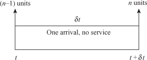
Figure 11.12
The product of these probabilities is given by
Pn−1(t)(λδt)(1 − μδt) = λP n−1(t)δt + 0(δt)(11.57)
- Product of the following three probabilities (Figure 11.13):

Figure 11.13
Probability that
- There are (n + 1) units in the system at time t = Pn+1(t).
- There is no arrival during the time interval δt = P0(δt) = λδt
- There is one service during the time interval δt = φδt(1)μδt
The product of these probabilities is given by
Pn+1(t) = (1 − λδt)(μδt) = Pn+1(t)μδt + 0(δt)(11.58)
By adding the above three independent compound probabilities Eqs. (11.56–11.58), we obtain the probability of n units in the system at time t + δt:
Pn(t + δt) = Pn(t)[1 − (λ + μ) δt] + Pn−1(t)λδt + Pn+1(t)μδt + 0(δt)
Transposing, dividing both sides by δt and taking limits as δt → 0
![]() (11.59)
(11.59)
![]() (11.60)
(11.60)
![]()
In the same way, the probability that there will be no unit, n = 0, in the system at time t + δt will be the sum of the following two independent probabilities.
Probabilities that
- There is no unit in the system at time t and no arrival in time δt = P0(t) + (1 − λδt)
- There is no unit in the system at time t, one unit served in δt and no arrival in δt
= P1(t) + (1 − λδt)(μδt)) = P1(t)μδt + 0(δt)(11.61)
Adding these two probabilities, we have
P0(t + δt) = P0(t)(1 − λδt) + P1(t)μδt + 0(δt)(11.62)
Now
![]() (11.63)
(11.63)
![]()
When we consider steady-state imposing the conditions
![]() (11.64)
(11.64)
where Pn is independent of time.
Consequently, the steady-state difference equations obtained are
− (λ + μ)Pn + λPn−1 + μPn+1 = 0 for n > 0(11.65)
λP0 + μP1 = 0 for n = 0(11.66)
11.10.2 Solution of the System of Difference Equations of Model 1
We have to solve the system of difference equations
−λP0 + μP1 = 0 for n = 0(11.67)
− (λ + μ)Pn + λPn−1 + μPn+1 = 0 for n > 0(11.68)
These equations can be written as
![]() (11.69)
(11.69)
![]() (11.70)
(11.70)
We will prove by induction that
![]() (11.71)
(11.71)
For n = 0, it is obvious. For n = 1, it is true by Eq. (11.69). Assume that Eq. (11.71) holds for n = 0, 1, 2, …, (m − 1) and m.
So that we have among other equations
![]() (11.72)
(11.72)
![]() (11.73)
(11.73)
Replacing n by m in Eq. (11.71), we have
![]()
![]()
![]()
This proves by induction that Eq. (11.71) holds for n = 0, 1, 2, …
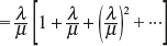
Now, using the fact that ![]() Pn = 1, we obtain
Pn = 1, we obtain
![]() (11.74)
(11.74)
since arrival rate (λ) < service rate (μ) and the infinite geometric progression.
Substituting the value of P0 at Eq. (11.74) into Eq. (11.71), we get
![]() (11.75)
(11.75)
where ![]()
Equations (11.74) and (11.75) give the required probability distribution of queue length.
11.10.3 Measures of Model 1
- To find the expected (average) number of units in the system Ls By definition of the expected value:


 (11.76)
where
 is the sum of infinite GP with CR
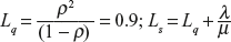
- To find the expected (average) queue length Lq There are (n − 1) units in the queue excluding the one being serviced:

 (11.77)


- To find the mean (or expected) waiting time in the queue (excluding the service time) Wq The expected time spent in queue is given by


 (11.78)
- To find the expected waiting time in the system (including service time Ws
Ws = Expected waiting time in the system
= Expected waiting time in queue + expected service time

expected service time or mean service time

- To find the expected waiting time of a customer who has to wait (W | W > 0) The expected length of the busy period is given by


 (11.79)
where

- To find the expected length of non-empty queue (L | L > 0) By the conditional probability, (L | L > 0) = Ls/P (an arrival has to wait; L > 0)
= Ls/(1 − P0) (∵ probability of an arrival not to wait is P0)
 (11.80)
 - To find the variance of queue length


 (11.81)

Let s = 1 + 22ρ + 32ρ 2 + …
Integrating both sides w.r.t. ρ from 0 to ρ

Now differentiating w.r.t ρ

- To find the probability of arrivals during the service time of any given customer
The arrivals are Poisson and service times are exponential. So, the probability of r arrivals during the service time of any specified customer is given by


 (11.82)
11.10.4 Inter-relations between Ls, Lq, Ws, Wq
It can be established under general conditions of arrival, departure and service discipline that
Ls = λWs(11.83)
Lq = λWq(11.84)
hold. By definition,
![]() (11.85)
(11.85)
Multiplying both sides of this equation by λ and using the above general relations, we get
![]()
Example 11.1
In a railway marshalling yard, goods trains arrive at the rate of 30 trains/day. Assuming that the inter-arrival time follows an exponential distribution and the service time (the time taken to hump a train) distribution is also exponential with an average 30 min.
Calculate
- Average number of trains in the queue.
- Probability that the queue size exceeds 10
If the input of trains increases to an average 33 trains/day, what will be change in (a) and (b)? Establish the formula you use in your calculations.
Solution Here
![]()
![]()
![]()

- P(queue size ≥ 10) = ρ10 = (0.75)10 = 0.06
When the input increases to 33 trains/day,
λ = 1/43, μ = 1/36
∴ ρ = λ/μ = 36/43 = 0.84
Then,

- P(queue size ≥ 10 ) = (0.84)10 = 0.2
Example 11.2
In Example 11.1, calculate
- Expected waiting time in the queue
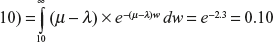
- Probability that the number of trains in the system exceeds 10
- Average number of trains in the queue
Solution ![]()
- Expected waiting time in the queue

- P(queue size ≥ 10) = ρ10 = (0.75)10 = 0.06

= 2.25 or 2 trains
Example 11.3
A TV repairman finds that the time spent on his jobs has an exponential distribution with mean 30 min. If he repairs sets in the order in which they come in and if the arrival of sets is nearly Poisson with an average rate of 10 per an 8-h/day, what is the repairman’s expected idle time each day? How many jobs are ahead of the average set just brought in?
Solution ![]()
∴Expected numbers of jobs are

![]()
The fraction of hours for which the repairman is busy (i.e. traffic intensity) is λ/μ.
The number of hours for which the repairman remains busy in an 8h/day
![]()
The time for which the repairman remains idle in an 8-h/day = 8 − 5 = 3 h.
Example 11.4
At what average rate must a clerk at a super market work in order to ensure a probability of 0.90 that the customer will not have to wait longer than 12 min. It is assumed that there is only one customer to which customers arrive in a Poisson fashion at an average rate of 15 per hour. The length of service by the clerk has an exponential distribution.
Solution Here
![]()
P(waiting time ≥ 12) = 1 − 0.90 = 0.10
![]()
![]()
![]()
Example 11.5
Arrivals at a telephone booth are considered to be Poisson with an average time of 10 min between one arrival and the next. The length of a phone call assumed to be distributed exponentially with mean 3 min.
- What is the probability that a person arriving at the booth will have to wait?
- What is the average length of the queues that form from time to time?
- The telephone department will install a second booth when convinced that an arrival would expect to have to wait at least 3 min for the phone. By how much the flow of arrival be increased in order to justify a second booth?
Solution ![]()
-

-

-

Since Wq = 3,
 and λ = λ′ (for second booth), we have
  ⇒ λ′ = 0.16
∴ Increase in the arrival rate = 0.16 − 0.10 = 0.06 arrivals/min.
Example 11.6
In Example 11.5, a telephone booth with Poisson arrivals spaced 10 min apart on the average and exponential call lengths averaging 3 min.
- What is the probability that an arrival will have to wait more than 10 min before the phone is free?
- What is the probability that it will take him more than 30 min altogether to wait for phone and complete his call?
- Estimate the fraction of a day that the phone will be in use.
- Find the average number of units in the system.
Solution Here λ = 0.1 arrival/min and μ = 0.33 service/min
![]()
- P(waiting time ≥ 10)

- P(waiting time in the system ≥ 10)

- The fraction of a day that the phone will be busy (i.e. traffic intensity) is

- Average number of units in the system is

11.10.5 Model 2(A)—general Erlang Model (M|M|1):(|FCFS) (Birth and Death Process)
To Obtain the System of Steady-state Equations Let λ = λn be the arrival rate and μ = μn be the service rate depending upon n.
Then proceeding as in the case of model 1, we get
![]() (11.86)
(11.86)
![]() (11.87)
(11.87)
Dividing by δt, transposing and taking the limit as δt → 0, we obtain
![]() (11.88)
(11.88)
![]() (11.89)
(11.89)
Taking ![]() in the steady state, we obtain
in the steady state, we obtain
![]() (11.90)
(11.90)
![]() (11.91)
(11.91)
11.10.6 Solution of the System of the Difference Equations of Model 2(A)
From Eq. (11.91), we get
![]() (11.92)
(11.92)
From Eq. (11.90), we get
![]() (11.93)
(11.93)
![]()
![]() (11.94)
(11.94)
Generally, we obtain
![]() (11.95)
(11.95)
Since ![]()
![]()
![]() (11.96)
(11.96)
![]()
The series is meaningful only if it is convergent.
Case 1: (λn = λ, μn = μ) In this case,

![]()
![]() (11.97)
(11.97)
which is exactly the result we have obtained for model 1.
Case 2: ![]() In this case, the arrival rate λn depends on n inversely and the rate of service μn is independent of n. It is called the case of queue with discouragement.
In this case, the arrival rate λn depends on n inversely and the rate of service μn is independent of n. It is called the case of queue with discouragement.
Now
![]()
![]()
![]()
![]() (11.98)
(11.98)
In this case, Pn follows the Poisson distribution where ![]() = ρ is constant: ρ > 1 but finite.
= ρ is constant: ρ > 1 but finite.
Case 3: (λn = λ, μn = μ) This is a case of infinite stations. In this case,
![]()
![]() (11.99)
(11.99)
![]()
which follows the Poisson distribution law.
Example 11.7
Problems arrive at a computing centre in a Poisson fashion at an average rate of 5 per day. The rules of the computing centre are that any man waiting to get his problem solved must aid the man whose problem is being solved. If the time to solve a problem with one man has an exponential distribution with mean time of ![]() day, and if the average solving time is inversely proportional to the number of people working on the problem, approximate the expected time in the centre for a person entering the line.
day, and if the average solving time is inversely proportional to the number of people working on the problem, approximate the expected time in the centre for a person entering the line.
Solution Here λ = 5 problems/day and μ = 3 problems/day (mean service rate with one unsolved problem).
The expected number of persons working at any specified instant is ![]()
where ![]() (Case 2)
(Case 2)
![]()
![]()
Substituting the value of λ and μ, we get
![]()
The average solving time which is inversely proportional to the number of people working on the problem is ![]() day/problem.
day/problem.
∴ Expected time for a person entering the line is
![]()
11.10.7 Model 3 (M |M |1):(N|FCFS)
Consider the case where the capacity of the system is limited, say N.
The physical interpretation for this model is that
- There is room only for N units in the system (as in a parking lot) or
- Arriving customers will go for their service elsewhere permanently, if the waiting time is too long (≤ N)
To Obtain Steady State Difference Equations The simplest way of deriving the equation is to treat the present model as a special case of Model 2 where
![]()
μn = μ for n = 1, 2, 3, …
Now, following the derivation of equation in Model 1, we get
![]() (11.100)
(11.100)
![]() (11.101)
(11.101)
![]() (11.102)
(11.102)
Dividing the equations by δt and taking the limit as δt → 0, we get
![]() (11.103)
(11.103)
![]() (11.104)
(11.104)
![]() (11.105)
(11.105)
In the case of steady state, as t → ∞ and Pn(t) → Pn (independent of t) and hence P′n(t) → 0, we obtain
![]() (11.106)
(11.106)
![]()
![]() (11.107)
(11.107)
![]() (11.108)
(11.108)
11.10.8 Solution of the System of Difference Equations of Model 3
![]() (11.109)
(11.109)
![]() (11.110)
(11.110)
Generally,
![]() (11.111)
(11.111)
n = N, PN+1 = 0(11.112)
We have
![]()
![]() (11.113)
(11.113)
Substituting the values of P0 into
![]()
for x = 0, 1, 2, …, n(11.114)
Measures of Model 3
![]()
![]() (11.115)
(11.115)
![]() (11.116)
(11.116)
![]() (11.117)
(11.117)
![]() (11.118)
(11.118)
Example 11.8
If for a period of 2 h in a day (8–10 am) trains arrive at the yard every 20 min, but the service time continues to remain 36 min, then calculate for this period
- Probability that the yard is empty
- Average queue length
on the assumption that the time capacity of the yard is limited to 4 trains only.
Solution ![]()

- Average queue size

= (0.04)(ρ + 2ρ2 + 3ρ3 + 4ρ4)
= 0.04 × 72.0 = 2.9 ≅ 3 trains
EXERCISES
- 1. What is a queueing theory problem?
- Explain a queueing system. What is meant by transient and steady of a queueing system?
- Describe the basic elements of a queueing system.
- Show that the number of arrivals n in a queue in time t follows the Poisson distribution, stating the assumptions clearly.
- Show that the distribution of the number of births up to time t in a simple birth process follows the Poisson law.
- Explain what do you mean by Poisson process. Derive the Poisson distribution, given that the probability of single arrival during a small time interval st is λst and that of more than one arrival is negligible.
- Show that if the inter-arrival times are negative exponentially disturbed, the number of arrivals in a time period is a Poisson process and conversely.
- State that in the three axioms underlying the exponential assumptions, can two events occur during a very small interval.
- Establish the probability distribution formula for pure death process.
- Explain Kendall’s notations for representing queueing models.
- Explain (M|M|1):(∞|FCFS) queueing model. Derive and solve the difference equations in steady state of the model.
- Explain (M|M|1) queue model in the transient state. Derive steady-state difference equations and their solutions.
- Show that average number of units in an (M|M|1) model is.
- Discuss (M|M|1):(∞|FCFS) queueing model and find the expected line length E(Ls) in the system.
- For the (M|M|1) queueing system, find
- Expected value of queue length n
- Probability distribution of waiting time w.
- A telephone booth functions with Poisson arrivals spaced 10 min apart on the average, and exponential call length averaging 3 min.
- What is the probability that an arrival will have to wait more than 10 min before the phone is free?
- What is the probability that it will take a customer more than one 10 min altogether to wait for phone and complete his call?
- Estimate the fraction of a day that the phone will be in use.
- Find the average number of units in the system.
Ans: (a) 0.03, (b) 0.10, (c) 0.3 and (d) 0.43 customer
[Hint: (a) λ = 0.1 and μ = 0.33
P(waiting time ≥


(b) P(waiting time ≥
(c) Traffic intensity

(d)

= 0.43 customer]
- The inter-arrival times at a service centre are exponential with an average time of 10 min. The length of the service time is assumed to be exponentially distributed with mean 6 min. Find
- Probability that a person arriving at the booth will have to wait.
- Average length for the queue that forms and the average time that an operator spends in the queueing system.
- Manager of the centre will install a second booth when an arrival would have to wait 10 min or more for the service. By how much must the rate of arrival be increased in order to justify a second booth?
- Probability that an arrival will have to wait for more than 12 min for service and to obtain tools.
- Probability that there will be 6 or more operators waiting for service.
Ans: (a) 0.6, (b) 1/4 h, (c) λ = 6.25 and μ = 60, (d) 0.27 and (e) (0.6)6
[Hint: (a) Probability of waiting = 1 − p0

(b)

(c)


(d)


(e) Probability of six or more operators waiting for service = ρ6 = (0.6)6]
- A company distributes its products by trucks loaded at its only loading station. Both company’s trucks and constructor’s trucks are used for this purpose. It was found out that on an average every 5 min, one truck arrived and the average loading time was 3 min. 50% of the trucks belong to the contractor. Find
- Probability that a truck has to wait
- Waiting time of a truck that waits
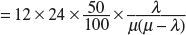
- Expected waiting time of constructor’s trucks per day, assuming a 24-h shift
Ans: (a) 0.6, (b) 7.5 min and (c) 10.8 h
[Hint: Here
(a) Probability that a truck has to wait
(b)
(c) Expected time of contractor’s truck per day
= (Number of trucks/day) × (Contractor’s percentage) × (Expected waiting time of a truck)
- A road transport company has bus reservation clerk on duty at a time. He handles information of bus schedules and makes reservations. Customers arrive at a rate of 8 per hour and the clerk can service 12 customers on an average per hour. After starting your assumptions, answer the following:
- What is the average number of customers waiting for the service of the clerk?
- What is the average time a customer has to wait before getting the service?
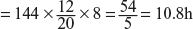
Ans: (a) Ls = 2 and Lq = 1.33, and (b) 15 min
[Hint: Here λ = 8 and μ = 12
(a)

(b)

FILL IN THE BLANKS
- FCFS means _____.
Ans: first come, first served
- FILO means _____.
Ans: first in, last out
- FIFO means _____.
Ans: first in first out
- LIFO means _____.
Ans: last in first out
- SIRO means _____.
Ans: service in random order
- A customer leaves the queue because the queue is too long and he has no time to wait. This type of customer’s behaviour is called _____.
Ans: balking
- The customer leaves the queue due to impatience. This type of customer’s behaviour is called _____.
Ans: reneging
- In certain applications, some customers are served before others regardless of their order of arrival. Thus, some customers are shown _____ over others.
Ans: priority
- Customers change from one waiting line to another shorter line. This behaviour is called _____.
Ans: jockeying
- The term _____ refers to the arrival of a new calling unit in the queuing system.
Ans: birth
- The term _____ refers to the departure of a severed unit.
Ans: death
- If x is the number of arrivals during time interval t, then the law of probability in Poisson process is given by px(b) = _____.
Ans:
- In Question 12, the term λt is the _____.
Ans: parameter
 _____.
Ans: 1
- P0 = _____.
Ans:

- Pn = _____.
Ans:

- Ls = _____.
Ans:

- Lq = _____.
Ans:

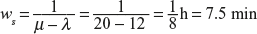
- ws = _____.
Ans:

- 20. wq = _____.
Ans:
