The first thing that we need to do is import all the Python libraries that we need. The last line of code—%matplotlib inline—is required only if you are running the code in IPython Notebook.

import pandas as pd
import numpy as np
import matplotlib as plt
import matplotlib.pyplot as plt
%matplotlib inline

Next we define a variable for the full path to our data file. It's recommended to do this so that if the location of your data file changes, you have to update only one line of code.

data_file = '/Users/robertdempsey/Dropbox/private/Python Business Intelligence Cookbook/Data/ISL/Advertising.csv'

Once you have the data file variable, use the read_csv() function provided by Pandas to create a DataFrame from the CSV file:

ads = pd.read_csv(data_file,
                        sep=',',
                        header=0,
                        index_col=False,
                        parse_dates=True,
                        tupleize_cols=False,
                        error_bad_lines=False,
                        warn_bad_lines=True,
                        skip_blank_lines=True,
                        low_memory=False
                        )

If using IPython Notebook, use the head() function to view the top five rows of the DataFrame. This helps to ensure that the data is imported correctly:

ads.head()

Since this is a new dataset, get a full list of the columns and data types in the DataFrame:

ads.dtypes

Use the shape method to find out the amount of data that the DataFrame contains:

ads.shape

Next we visualize the relationship between Sales and TV in a scatterplot. To do this, we use the plot() method of the DataFrame, specifying the kind of graph we want (scatter), the column to use for the x axis (TV), the column to use for the y axis (Sales), and the figure size (16x8):

ads.plot(kind='scatter',
         x='TV',
         y='Sales',
         figsize=(16, 8))

The resulting plot looks like the following image:

After that, we import the Python libraries we need to create a linear regression. For this, we import LinearRegression from the linear_model part of scikit-learn:

from sklearn.linear_model import LinearRegression

Next, create an instance of the LinearRegression model:

lm = LinearRegression()

After that, create a features array and assign the values of those columns to x. Then, add the values of the Sales column to y. Here I've chosen to use x and y as my variables; however, you could use any variable names you like:

features = ['TV', 'Radio', 'Newspaper']
x = ads[features]
y = ads.Sales

Next we fit the data to the model, specifying x as the data to fit to the model and y being the outcome that we want to predict.

lm.fit(x, y)

Next, print the intercept and coefficients. The intercept is the expected mean value of Y when all X=0.

print(lm.intercept_)
print(lm.coef_)

After that, we aggregate the feature names and coefficients to create a single object. We do this as a necessary first step in measuring the accuracy of the model:

fc = zip(features, lm.coef_)

This next line prints out the aggregate as a list:

list(fc)

Next we calculate the R-squared value, which is a statistical measure of how close the data is to the fitted regression line. The closer this number is to 100 percent, the better the model fits the data.

lm.score(x, y)

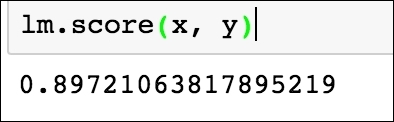
89 percent accuracy is very good!

Finally, we make a sales prediction for a new observation. The question we're answering here is: given the ad spend for three channels, how many thousands of widgets do we predict we will sell? We pass in the number of dollars (in thousands) spent on TV, radio, and newspaper advertising, and are provided with a prediction of the total sales (in thousands):

lm.predict([75.60, 132.70, 34])