6.4 Implementation issues

Search in book...
Toggle Font Controls
Create new playlist

Name your new playlist

Playlist description (optional)
Sign In

Email address

Password

Forgot Password?

or

Continue with Facebook

Continue with Google
Sign Up

Full Name

Email address

Confirm Email Address

Password

or

Continue with Facebook

Continue with Google

Figure 6.32 Overview of model used for describing the agricultural and silvicultural sectors in a scenario for future integrated food and energy production.

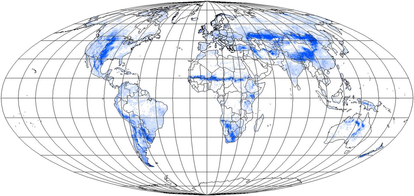
In the 2050 scenario, the land area used for food crops is considered the same as now. This includes the cropland area fraction (Fig. 6.33; AF in Fig. 6.32) and, for grazing, rangeland as well (Fig. 6.34). Forest (Fig. 6.35) and marginal land (Fig. 6.36) is not used for food crops. Some marginal land is used today for grazing in a less-intensive way, in contrast to the use of cropland in rotation for occasional grazing. In some areas (e.g., Africa), crop cultivation on the cropland fraction is little intensive, and present yields strongly reflect the agricultural practices of each region. As an indication of the potential biomass production in these areas, the model shown in Fig. 6.32 uses calculated net primary production data from the Terrestrial Ecosystem Model (TEM) of the Woods Hole group (Melillo and Helfrich, 1998; model evolution and description in Raich et al., 1991; Melillo et al., 1993; McGuire et al., 1997; Sellers et al., 1997), shown in Fig. 3.99. Global warming may induce increased primary production in a fairly complex pattern and the borders of natural vegetation zones are expected to change, sometimes by several hundred kilometers (IPCC, 1996).

Figure 6.33 The fraction of area used as cropland and cropland in rotation (taken as a fraction of each 0.5°×0.5° grid cell used for these purposes, on the basis of the classification of land cover in the U.S. Geological Survey (1997). See also Loveland *et al*. (2000).

Figure 6.34 The fraction of area used as rangeland (cf. Fig. 6.33).

Figure 6.35 The fraction of area occupied by forest (cf. Fig. 6.33).

Figure 6.36 The fraction of area considered marginal land (cf. Fig. 6.33).

Global warming–induced changes in area fractions are not included in the model, assuming that farming practice is able to gradually change and replace the crops cultivated in response to altered conditions, which are, in any case, long-term changes compared to the lifespans of annual crops. The model does not specify which crops will be cultivated at a given location, but simply assumes productivity consistent with growing crops suited for the conditions. The TEM data are for a mature ecosystem, taking into account natural water, humidity, and nutrient constraints, along with solar radiation and temperature conditions. Annual crops are likely to have smaller yields because of only partial ground cover during part of the year and the corresponding smaller capture of radiation. On the other hand, the crops selected for cultivation may be favorably adapted to the conditions and therefore may give higher yields than the natural vegetation at the location. Furthermore, irrigation may prevent yield losses in dry periods, and application of chemical fertilizers may improve overall yields.

It is conceivable that ecological concern will dictate restricted use of these techniques and will lead to increased use of organic agricultural principles, which are currently used in about 10% of agricultural areas in Europe and a few other places. The 2050 scenario assumes what is called integrated agriculture (Sørensen et al., 1994), a concept that includes a ban on pesticide use and that encourages use of recycled vegetable residues and animal manure for nutrient restoration, but that does not exclude biological pest control and limited use of chemical fertilizers. The yield losses associated with integrated agriculture are under 10% of current chemical-based agriculture yields, according to experience in Northern Europe.

On cultivated land (including grazing land and managed forests) in regions like Denmark (modest solar radiation and good soil and water access), the average annual biomass production is 0.62 W m⁻² (of which 0.3 W m⁻² are cereal crops; Sørensen et al., 1994). This equals the value for a grid cell in Denmark given in the TEM database for mature natural productivity. In Southern Europe, current production is about half (Nielsen and Sørensen, 1998), while the TEM database gives a slightly higher value than for Denmark. The reasons for this are less intensive agricultural practice and water limitations for the growth pattern of the crops cultivated (limitations that would be less severe for a mature ecosystem). Therefore, it seems reasonable to use the TEM in the scenario as a proxy for cultivation yields, provided that one assumes improved farming techniques by the year 2050 and assumes that irrigation and chemical fertilizers are used when necessary. This is precisely the assumption stated above as the basis for the scenario. The model then uses the net natural primary production data of the TEM globally, but without adding further increases on the basis of irrigation (which in dry regions can double agricultural output) and use of chemical fertilizers (which can provide a further doubling, if the soil is poor in nutrients or nutrients are not returned to the fields). In other words, the disadvantage of going from mature vegetation to annual crops is offset by the advantage of reduced limiting factors related to water and nutrients. In Fig. 6.32, this means disregarding the irrigation and fertilizer parameters IF and FI and proceeding with the potential production PP taken from the TEM database.

The TEM global biomass production estimates for PP shown in Fig. 3.99 are expressed in energy units (1 g carbon per year is equal to a rate of energy production of 0.00133 W).

Currently, in Denmark only about 10% of this energy is contained in food consumed domestically, which indicates that there is room for altered management of the system, by diverting residues to energy extraction and later returning nutrients to the fields. One may also note that the current system is based on high meat consumption and the associated emphasis on raising livestock and, in the Danish case, export. Even the modest change in the vegetable to animal food consumption ratio that is assumed in the demand scenario shown in Figs. 6.5 and 6.6 shows that it is possible globally to divert substantial amounts of biomass to energy purposes without jeopardizing the ability to provide food for a growing world population.

It is not assumed that the intensive agricultural practices of Northern Europe will have been adopted globally by year the 2050. The agricultural efficiency factor AE in Fig. 6.32 is taken as unity only for regions 1 and 2 (cf. Table 6.3). For Africa (region 6) it is taken as 0.4, and for the remaining regions it is taken as 0.7. The fraction of the biomass production actually harvested is taken globally as HF=0.4. The remaining fraction consists of roots and residues plowed under in order to provide natural fertilization for the following growth season.

For land areas classified as cropland, the assumed distribution of uses is given in Table 6.7, based on considerations of cropland scarcity and traditional practices in livestock raising. The low animal fodder value in Africa reflects the fact that the African tradition is to raise livestock on rangeland, not to use cropland to provide fodder.

Table 6.7

Parameters used for cropland biomass production in the 2050 scenario (Regions are defined in Table 6.2; see also Fig. 6.32 for explanation of abbreviations.)

Region	AE (Cropland)	HF	UF (Vegetable Food)	UF (Fodder)	UF (Energy Crops)
1	1	0.4	0.4	0.5	0.1
2	1	0.4	0.4	0.5	0.1
3	0.7	0.4	0.5	0.5	0
4	0.7	0.4	0.4	0.5	0.1
5	0.7	0.4	0.7	0.3	0
6	0.4	0.4	0.8	0.2	0

The amounts of vegetable-type food that can potentially be produced and delivered to end-users in this scenario can now be calculated on an area basis, assuming the losses in going from vegetable food produced to vegetable food delivered as 25% [IE(veg. products)=0.75 for vegetable food products in Fig. 6.23],

$Delivered vegetable food = A F (c r o p l .) \times P P [W m^{- 2}] \times A E \times H F \times U F (v e g . f o o d) \times I E (v e g . p r o d u c t s),$ $Delivered vegetable food = A F (c r o p l .) \times P P [W m^{- 2}] \times A E \times H F \times U F (v e g . f o o d) \times I E (v e g . p r o d u c t s),$

where AF and PP depend on the precise geographic location and the others only on region. The calculated distribution of vegetable food delivered to consumers is shown in Fig. 6.37.

Figure 6.37 Potential delivery to final consumer of vegetable-based food from cropland production, expressed in units of energy flow (W m⁻²).

For food from animals, such as meat, milk, and eggs, the average efficiency in transforming biomass to delivered animal products is assumed to be IE(animal products)=0.15, a value reflecting a typical average of a smaller efficiency for meat production and a higher one for milk and eggs (Sørensen et al., 1994). The amount of animal-based food using cropland-derived fodder and delivered to the consumer is thus

$Delivered animal food (1) = A F (c r o p l .) \times P P [W m^{- 2}] \times A E \times H F \times U F (f o d d e r) \times I E (animal products) .$ $Delivered animal food (1) = A F (c r o p l .) \times P P [W m^{- 2}] \times A E \times H F \times U F (f o d d e r) \times I E (animal products) .$

The distribution of potential animal food deliveries based on livestock being fed fodder produced on cropland is shown in Fig. 6.38.

Figure 6.38 Potential delivery to final consumer of animal-based food from livestock being fed with fodder grown on cropland, in energy units.

The other part of animal food is from animals grazing on rangeland, where we shall assume that livestock grazes HF=0.4 of the biomass production per unit of area, and put AE=1. The use of rangeland is assumed to be 50% for grazing and 50% for other purposes (such as energy crops or no commercial use). Thus, the utilization factor is taken as UF(grazing)=0.5:

$Delivered animal food (2) = A F (r a n g e l a n d) \times P P [W m^{- 2}] \times H F \times U F (g r a z i n g) \times I E (animal production) .$ $Delivered animal food (2) = A F (r a n g e l a n d) \times P P [W m^{- 2}] \times H F \times U F (g r a z i n g) \times I E (animal production) .$

The distribution of potential animal food deliveries to end-users based on rangeland grazing is shown in Fig. 6.39. The ratio of the two contributions (crop feeding and rangeland grazing) is determined by the area set aside for each. The resulting fraction of animal food derived from rangeland grazing is 37%, in terms of energy content.

Figure 6.39 Potential delivery to final consumer of animal-based food from livestock grazing on rangeland, expressed in units of energy flow (W m⁻²).

The efficiency of the end-user’s making use of delivered food, denoted EE in Fig. 6.32, is for all bioenergy routes included in the definition of gross demand in section 6.2.3.

6.3.4 Biofuel production

A number of fuels may be produced from biomass and residues derived from vegetable and animal production or from forestry and dedicated energy crops. They range from fuels for direct combustion over biogas (mainly methane mixed with carbon dioxide) to liquid biofuels, such as ethanol and methanol, or gaseous fuels, such as synthesis gas (a mixture of mainly carbon monoxide and hydrogen, also being an intermediate step in producing methanol) or pure hydrogen. The production of biofuels by thermochemical processes is based on high-temperature gasification and various cleaning and transformation processes (Jensen and Sørensen, 1984; Nielsen and Sørensen, 1998).

Whether biofuel production is by thermal or biological processes, the expected conversion efficiency is of the order of FE=50% (cf. Fig. 6.32). This is to be compounded with a factor describing the ability of the biofuel industry to collect the necessary feedstock. This collection-efficiency factor, which we call CF, describes the efficiency in collecting biomass for industrial uses. For vegetable foods, it is assumed that CF(veg. waste)=25% of the gross production is available for energy production [some of this would come from food-industry losses of (1−IE(veg. prod.))=25%, and some from the subsequent household losses of 30%; cf. sections 6.2.3 and 6.3.3]. The overall yield of biofuels from vegetable crops is then

$Biofuels from vegetable foodcrops = A F (c r o p l .) \times P P [W m^{- 2}] \times A E \times H F \times U F (v e g . f o o d) \times C F (v e g . w a s t e) \times F E .$ $Biofuels from vegetable foodcrops = A F (c r o p l .) \times P P [W m^{- 2}] \times A E \times H F \times U F (v e g . f o o d) \times C F (v e g . w a s t e) \times F E .$

Of course, manure is available only when livestock are kept in stables or similar areas that allow easy collection. The model assumes that grazing animals leave manure in the fields and that it is not collected (although it could be in some cases), but that animals being fed fodder from crops will be in situations where collection of manure is feasible. Furthermore, although the 85% of animal biomass not ending up in food products will be used both to maintain the metabolism of livestock and the process of producing manure, it will also contain a fraction that may be used directly for fuel production (e.g., slaughterhouse wastes). Combined with manure, this is considered to amount to CF(anim.)=0.6, giving, for the fodder-to-animal route to biofuels:

$Biofuels from manure and other animal residues = A F (c r o p l .) \times P P [W m^{- 2}] \times A E \times H \times U F (f o d d e r) \times (1 - I E (a n i m . p r o d .)) \times C F (a n i m .) \times F E$ $Biofuels from manure and other animal residues = A F (c r o p l .) \times P P [W m^{- 2}] \times A E \times H \times U F (f o d d e r) \times (1 - I E (a n i m . p r o d .)) \times C F (a n i m .) \times F E$

The possibility of producing biofuels from forestry residues (either scrap derived from the wood industry or residues collected as part of forest management) may be described by a factor CF(forestry)=0.3, defined as a percentage of the total forest biomass production. This is the fraction collected, expressed in energy units. For managed forests, it depends on the fraction of wood suitable for the wood manufacturing industry (furniture, etc.), which depends on the tree type. Adding wood scrap from industry and discarded wooden items, as well as residue from forest management, would in many regions exceed 30%. However, starting from an enumeration of all forests, including the rainforests and other preservation-worthy forest areas that are not proposed to be touched, and considering only managed forests that deliver to wood industries, 30% is probably a maximum for the year 2050. The forest-residue-to-biofuel route is then

$Biofuels from forest management = A F (f o r e s t l a n d) \times P P [W m^{- 2}] \times H F \times C F (f o r e s t r y) \times F E .$ $Biofuels from forest management = A F (f o r e s t l a n d) \times P P [W m^{- 2}] \times H F \times C F (f o r e s t r y) \times F E .$

The potential amounts of biofuels that could be derived from forestry are shown in Fig. 6.40, and the sum of the three routes to biofuels described above are given on an area basis in Fig. 6.41. This may be called decentralized fuel production, although forestry may not be seen as entirely decentral in nature. However, forestry is an ongoing activity that is distinct from producing biofuels from land used exclusively for energy crops. Two energy-crop routes are considered.

Figure 6.40 Potential delivery to final consumer of biofuels based on forestry residues and wood waste, expressed in energy units.

Figure 6.41 Potential delivery to final consumer of all “decentralized” biofuels based on forestry, agricultural residues, manure, and household waste, in units of energy flow (W m⁻²).

While the biomass production on rangeland does not give rise to biofuel production because manure from grazing livestock is not collected, some of the rangeland may be suited for cultivation of dedicated energy crops. Because only 50% of rangeland is assumed to be used for grazing, one may consider the remaining 50% a potentially exploitable area for energy purposes, in the scenario versions where centralized energy schemes are considered acceptable [i.e., UF(rangeland energy crops)=0.5]. For cropland, it is also assumed that a maximum of 10% is set aside for energy crops in areas with generous resources, such as Western Europe and the Americas [see the UF(cropland energy crops) values of 0.1 or 0 in Table 6.7]. The potential biofuel production from these areas is

$Biofuels from energy crops on cropland = A F (c r o p l .) \times P P [W m^{- 2}] \times A E \times H F \times U F (c r o p l a n d e n e r g y c r o p s) \times F E,$ $Biofuels from energy crops on cropland = A F (c r o p l .) \times P P [W m^{- 2}] \times A E \times H F \times U F (c r o p l a n d e n e r g y c r o p s) \times F E,$

$Biofuels from energy crops on rangeland = A F (r a n g e l a n d) \times P P [W m^{- 2}] \times H F \times U F (r a n g e l a n d e n e r g y c r o p s) \times F E .$ $Biofuels from energy crops on rangeland = A F (r a n g e l a n d) \times P P [W m^{- 2}] \times H F \times U F (r a n g e l a n d e n e r g y c r o p s) \times F E .$

The value of FE is 0.5. The area distribution for the two potential sources of biofuels from energy crops is shown in Fig. 6.42.

Figure 6.42 Potential delivery to final consumer of “centralized” biofuels based on dedicated energy crops grown on part of rangeland and minor parts of cropland, in energy units.

With increasing pressure for food production for an increasing world population, energy crops may well be considered unfeasible. On the other hand, increased food production also implies an increasing amount of residues becoming available for biofuel production. Furthermore, the currently rapid increase in aquaculture (for fish, shellfish, and vegetables based, e.g., on kelp) offers additional residues for energy production, and because the ocean areas are huge, the possibility of aquacultural energy crops is also not excluded. In fact, aquacultural biofuels are included in several of the scenarios constructed in section 6.6.

6.4 Implementation issues

Once demand has been determined and supply options mapped, there may still be more than one intermediate conversion system that will join the supply-and-demand requirements. They could be selected according to the criterion of minimal economic, environmental, and social impact (according to the evaluation methods presented in Chapter 7). Assuming this is done, there is a complete system in the hands of the planner, ready to be checked for consistency. Consistency is in part internal consistency, meaning that the system functions smoothly at all times and for all consumers, and in part consistency in the sense that the system condition can be reached from the present situation. Implementation studies usually end up quantifying a number of decisions that have to be made, at specified moments in time, in order for the development from the current state to the scenario state to happen.

Implementation evaluations have been made by first checking the technical consistency of the scenario system in the world assumed at the time envisaged for the scenario to be realized and subsequently specifying the path that has to be taken to get there (Sørensen, 1975 to 2008b and 2008c). An alternative method for an implementation study is backcasting, i.e., starting at the final scenario and working backward to the present, making notes of the decisions needing to be taken along the way (Robinson, 1982, 1988).

A few general remarks on intermediary system optimization and scenario consistency checking are made below, followed by several sections of examples on smaller and larger geographic scales.

6.4.1 System choice and optimization

A number of physical constraints are imposed on a given energy system, including the availability of different renewable energy sources in the geographic regions of interest; the characteristics of different system components, such as response time for changing the level of energy delivery; the delivery energy form, which may not be uniquely given by the nature of the load; and so on. Figure 6.43 provides some possible components of energy systems based on renewable resources. More details are in the scenarios presented in sections 6.5 to 6.7.

Figure 6.43 Example of the components of a supply–demand matching energy system based on renewable sources, with primary and secondary conversion processes, storage, and transmission.

The rated capacity of each component of the energy supply system will generally be determined by the maximum load expected to be demanded, with some adjustments made if the system includes stores and energy-exchange facilities, adapting system performance according to the expected time distribution of source fluxes and loads. Situations may arise in which not all incident energy can be converted, because the demand is already met and the stores (or those for a given energy form) are full. In this case, as well as in situations where different parts of the system would each be capable of satisfying the load, system operational problems arise. Regulation procedures would then have to be defined that could determine which converter to tune down or stop in cases of system overflow and which stores should be depleted first when more than one is available to serve a given load at a given time. Also strategies for exchange of energy between regions with different load structures (or time zones) offer possibilities for avoiding over- or underflow (Meibom et al., 1999). Because the system is non-linear, there is no simple way of optimizing it, although relative minima in cost or other parameters may be sought (Sørensen, 1996).

6.4.2 Consistency of simulation

The consistency of a given scenario is checked by performing a simulation, typically with 1-hour time steps, through 1 or more years. Realistic variations in demand are introduced, although the actual demands at a future scenario year are of course not known. Typically, one would take the present data with temporal variations and scale it to the scenario assumption for the total energy demanded, using the energy forms considered. More subtle extrapolations can be made if the scenario contains prescriptions for normative changes in society, such as altered consumption habits or work relations.

Taking note of the system performance at each step and allowing use of storage reservoirs and import/export options, one checks that the are no misses in supply–demand matching and adjusts the size of the system components downward or adds more (when possible), if there is unused or insufficient capacity. This constitutes the consistency check, and if system expansion beyond what can be achieved with the sources designated as potentially available is not required, then the system is labeled as realistic.

Ideally, the implementation study would also require consistency checks at least at selected stages along the path of establishing the system, taking into account phase-out of existing equipment (with consideration of the economic effects of too early retirement).

There may be other things to keep track of than just the technical performance of the system. If, for instance, the purpose of the scenario is to avoid greenhouse warming, then the reduction of CO₂ emissions along the timeline of implementation should be calculated. If a motivation for the scenario is to allow more energy-related decisions to become decentralized or even to reach the level of individual personal choice, then these are qualities to monitor. Decentralization may involve a choice between large, centralized primary energy production plants (which are also possible for renewable energy—think of desert photovoltaic systems or gigawatt offshore wind farms, not to mention dammed hydro stations) or smaller units placed closer to the users. At the extreme, every household may fully control its energy supply, e.g., by reversible fuel-cell installations capable of producing vehicle fuel and conversion of rooftop photovoltaic power to hydrogen or hydrogen to electricity, as needed.

6.5 Local systems

Renewable energy conversion systems or combinations of systems for use in different regions and in differently structured societies will very probably have to be different. The contribution of a single type of conversion in the system may depend on local resource availability. In the early phase, co-existence of renewable and non-renewable components is likely and it is important to make them work together. Often this offers the advantage that fossil-fuel systems can alleviate the need for dedicated energy stores for the renewable components, until the renewable energy contribution grows large. Solar thermal collectors would work well in some regions of the world, but, in other regions, it may be difficult to reach 100% coverage of heat needs during winter. The examples given in this section deal with some of these problems, which are of immediate interest for current implementations of energy supply systems, by investigating the relation between fractional load coverage and various system parameters characterizing the size and complexity of the system.

6.5.1 Solar heat or heat-and-electricity systems

The examples described in this subsection are based on flat-plate solar collector devices (cf. section 4.4.3) in various configurations, and the system simulations use the database for the Danish Reference Year, which is summarized in section 3.1.3 (e.g., in Fig. 3.17). It is clear that use of the same systems at latitudes with higher levels of solar radiation will improve performance and makes it possible to cover loads with smaller and less expensive systems. On the other hand, the simulation of solar energy systems at fairly high latitudes (56°N for the Danish reference data) raises a number of design problems, which may show up more clearly than for latitudes with higher and more stable solar input and smaller heating loads, but which may still be of general interest. In any case, the need for heating is higher at higher latitudes, making the optimization of systems for such use particularly relevant.

Systems involving solar thermal collection into a heat store (cf. Fig. 4.84) have a complex dynamic behavior, due to the direct influence on absorber performance of heat-storage temperature, collector fluid inlet temperature, and speed of circulation. Indirectly, the collector circuit is influenced by heat-storage temperature of load patterns governing the heat exchange between store and load circuits. If a photovoltaic part is present (thus forming a hybrid photovoltaic-thermal—PVT—system), its performance depends on the complex temperature behavior only through the temperature dependence of power production efficiency (cf. Fig. 4.56), which in any case is much weaker than that of the thermal collection part.

6.5.1.1 Model description

The system modeled (using the software package NSES, 2001) is a building with solar collectors, heat stores (which could be communal, i.e., common for several buildings or even part of a district heating system), and load patterns consisting of time profiles of the use of electricity, space heating, and hot water. The design of the building has to be specified in order to calculate heat losses and energy gains through passive features (such as windows), as does the activities in the building relevant for energy flows [occupancy, use of electric appliances and lighting, opening and closing of shutters (if any) in front of windows, etc.]. The external parameters include ambient temperature, wind speed, and solar radiation.

In case both thermal and electric energy are produced, the thermal absorber could be the back plate of a photovoltaic collector sheet, or the thermal collection could be from the airflow over the PV panel but below a transparent cover. In the first case, the heat-transfer fluid would typically be water, and, in the second, case it would be air. Heat collection in front of the PV panel could have negative effects, such as more hours with dew formation on the cover glass. Heat collection behind the PV panel could be lowered, if reflective back layers are used in the PV cell design to increase light capture probability by prolonging the radiation path-length within the cell.

The simulations reported below use the model described in section 4.4.3 for solar thermal collection and heat exchange in the collector–storage circuit. Details of the radiation data used in the numerical examples and the load description entering the modeling of the storage–load circuit are given in the following subsections.

Solar radiation data used

Radiation data are taken from a stream of reference year data for a position 56°N and 10°E (cf. section 3.1.3). The data are collections of hourly global and diffuse radiation covering a year and exhibiting variations typical of what is contained in 30-year meteorological time-series. A reference year (of which several have been constructed, covering cities in Europe and the United States) is put together by pieces of actual data from the 30-year data source (30 years is the selected time span for defining a “climate”). Typical segment length is 14 days, in order to preserve the short-term correlations in the data arising from continuity and the typical passage time of weather fronts. Thus, the data are supposed to have both the typical short-term correlations and the long-term variability that can ensure realistic modeling of solar system performances over the lifetime of the system in question.

The most recent* Danish reference year data set employed is illustrated in Figs. 6.44 and 6.45 and shows the hourly Danish 1996 reference year profiles for ambient temperature and solar radiation incident on a south-facing plane tilted 45°.

Figure 6.44 Danish 1996 reference year profile of ambient temperatures.

Figure 6.45 Danish 1996 reference year profile of 45°S solar radiation over the year.

The collection of short-wavelength radiation by the solar panel takes place in a system comprising one or several cover layers followed by one or more absorbing layers. If present, the photovoltaic modules constitute one layer. Part of the absorbed radiation is transformed into an electric current, while the rest is transformed into long-wavelength radiation, which is either converted into useful heat or lost to the surroundings.

In contemporary thermal solar collectors, a heat-transfer fluid is passed over or under the usually building-integrated solar collector. The connection with the rest of the system (heat-store and building loads), illustrated in Fig. 4.84, usually contains two circuits, called the collector and the load circuit, both connected to the heat store by heat exchangers.

The heat-transfer fluid is typically air or water. Use of water in PVT systems entails a requirement for sealed paths and protection against corrosion, just as for thermal solar collectors. Although the use of air as a transfer fluid is easier, the low heat capacity of air and low energy transfer rates to and from air limit its applicability.

Thermal collection in front of the solar cell (but below a cover glass) may alter the efficiency of the PV conversion in a negative way, whereas collection behind the solar cell should pose few problems once it has been ensured that the PV and thermal plate layers are well connected, so that heat transfer (conduction) is high. Incoming solar radiation is made useful for electricity production, is transformed into heat taken up by components of the collector, or leaves the cell through front or rear walls. A reflective rear layer may be used at the back of the PV module. It causes the light to pass through the solar cell twice, with a greater overall chance of capture. On the other hand, this excludes the possibility for light to pass through the PV layers and only to be absorbed in an underlying thermal collector layer (Sørensen, 2002).

6.5.1.2 Heat load of an individual house

The heat load of a building is fixed by specifying the indoor temperature of the building and the hot-water need as a function of time. The indoor temperature may need to be fixed, or it may be allowed to decrease during the night and when the house is unoccupied. For the purpose of simulation, the hot-water needs may be considered to be identical on every day of the year and concentrated in certain hours, such as a morning peak plus a period of moderate use in late afternoon and throughout the evening (including clothes washing, dish washing, baths, etc.). The amount of heat required to keep the indoor temperature at the prescribed value does not, on the other hand, remain constant throughout the year, but equals the heat losses through doors, windows, walls, floor, and roof, as well as losses associated with air exchange, which may be regulated by a ventilation system or may be entirely “natural,” i.e., associated with crevices and the like in building materials and assembly sites.

The heat losses through building surfaces depend on the difference between inside and outside temperature and may be approximated by a linear expression

$h = (T_{L} - T_{a}) \sum_{i} A_{i} U_{i},$ $h = (T_{L} - T_{a}) \sum_{i} A_{i} U_{i},$ (6.2)

(6.2)

where T_L is the indoor (“load-”) temperature, T_a is the outside temperature, and A_i and U_i are corresponding areas and specific heat-loss rates for different parts of the external building surface (walls, windows, roof, floor, etc.). The floor against the ground may be poorly described by the expression with T_a, and the heat-loss expression should perhaps contain a particular term describing the floor loss, being proportional to the difference between the load and soil temperatures, rather than the difference between the load and air temperatures. However, the heat-loss rates U_i are in any case only approximately constant, and they may have a further dependence on temperature (e.g., if radiative transfer is involved) and on outside wind speed, moisture, etc., as discussed above in connection with the collecting absorber.

An average contemporary one-family detached dwelling located in the temperate climatic zone may be characterized by wall and ceiling losses amounting to around 57 W °C⁻¹ (U_wall in W m⁻² °C⁻¹ times wall and ceiling total area) and ground floor losses of 18 W °C⁻¹ (U_floor often slightly lower than U_wall). With 20 m² window area and U_window=2 W m⁻² °C⁻¹ (two layers of glazing; with intermediate space filled with low-conduction gas, the value may be reduced to half), the total “conduction” loss becomes 115 W °C⁻¹. If the house has 1½ stories (cf. sketch in Fig. 6.46), the ground floor area may be about 100 m² and the combined floor area above 150 m² (depending on how low ceiling heights are accepted as contributing to floor area for the upper floor). This corresponds to an inside volume of about 330 m³, and if the rate of air exchange is 0.75 per hour, then V_air=250 m³ of air per hour will have to be heated from T_a to T_L (reduction is possible by letting the outgoing air preheat the incoming air in a heat exchanger),

${(A_{i} U_{i})}_{air exchange} = V_{a i r} C_{v}^{a i r} \approx 87 W ° C^{- 1},$ ${(A_{i} U_{i})}_{air exchange} = V_{a i r} C_{v}^{a i r} \approx 87 W ° C^{- 1},$

since $C_{v}^{a i r}$ $C_{v}^{a i r}$ =0.347 Wh m⁻³ °C⁻¹. For the reference calculation, V_air is taken as 250 m³ h⁻¹ only during the period 16:00 to 08:00 and as 125 m³ h⁻¹ between 08:00 and 16:00 (assuming lower occupancy during these hours and a programmable ventilation system). Measurements have suggested that the air-exchange rate in naturally ventilated Danish dwellings (individual houses as well as apartments) may be lower than required for reasons of health (Collet et al., 1976). In a sample of 81 dwellings, a range of air-exchange rates between 0.15 and 1.3 times per hour was found, with the average value 0.62 times per hour.

Figure 6.46 Heat-load data for a one-family dwelling, in terms of monthly averages of heat fluxes. The layout and dimensions of the house are indicated as an inset.

The minimum ventilation requirement has been quoted as 8 m³ h⁻¹/cap (Ross and Williams, 1975), but it may be more if the ventilation air is polluted by, for example, automobile exhaust or if tobacco smoking, open-air cooking, fireplace combustion, or similar practices take place on the premises. The value quoted would roughly correspond to the smallest values encountered in the Danish measurements, assuming that a family with 4–5 members occupies the dwelling. Although this minimum air exchange generously provides the necessary oxygen and removes CO₂ from the air the family breathes, it may not be sufficient to ensure health and well-being. Indeed, when “dust” or other particulate matter is abundantly injected into the air (e.g., from carpets or from activities taking place in the building), then increased ventilation is definitely required. Analyses of particulate matter from the air of private dwellings show the largest component is often pieces of human skin tissue. It should also be kept in mind that many building materials release gases (some of which have adverse effects on health) in substantial quantities, for at least the first few years after installation.

The heat required to compensate for the building’s heat losses may be distributed by a device (radiative and/or convective) with a heat-transfer area chosen in such a way that any expected load can be met. In earlier individual or district heating fuel-based systems, it was customary to work with high inlet temperatures (steam at 100°C, water at 80°C). This was lowered to about 60°C after the first oil crisis in 1973. The minimum working inlet temperature would be about 45°C for a water radiator system, whereas distribution based on air circulation may employ heat supply of temperature around 28°C. The latter choice is made in the present calculations, partly because it is suitable for solar systems aiming at coverage during as large a fraction of the year as possible and partly because efforts to decrease building heat losses through better insulation will make the capital costs of a water distribution system less appealing. For each of the heat exchangers, a temperature loss of 8°C is assumed.

Hot water is assumed to be required at a temperature 42°C above the inlet (waterworks) temperature, which in Denmark is taken as 8°C.

The metabolism of persons present within the house releases heat, corresponding to roughly 125 W per person as an average net heat transfer to the surroundings. The changing occupancy of the house, as well as the lower rate of metabolism during sleep and the higher one during periods of high activity, are modeled by a variation in the gains from persons, assumed to be of an identical pattern every day of the year, as specified in Table 6.8. In addition, the use of appliances that convert electricity or another form of energy (cookers, washing machines, dishwashers, lights, amplifiers, and other electronic equipment, etc.) contributes to indirect heat gains, since the various conversions in most cases result in the release of the entire energy in the form of heat inside the house. The contribution from cooking is reflected in the distribution of the heat releases from appliances over different hours of the day, the assumed pattern being also given in Table 6.8. The gain from lighting, assumed to be dominated by highly efficient bulbs, is assumed to be 100 W during 1 hour in the morning and 8 hours in the evening, except when the outside total solar radiation exceeds 50 W m⁻². Again, the use of more efficient equipment, including low electricity-consuming light bulbs, does have the effect of diminishing indirect contribution to space heating with time.

Table 6.8

Reference data for simulation of solar system for a Danish one-family house.

1. Building heat losses

Loss rate through surface (except windows) 75 W°C⁻¹.

Loss rate through windows (no shutters) 40 W°C⁻¹.

Ventilation air 250 m³ h⁻¹ from 16:00 to 08:00, 125 m³ h⁻¹ from 08:00 to 16:00.

Minimum inlet temperature required for space heating load, 28°C.

Indoor temperature 20°C from 07:00 to 09:00 and from 16:00 to 24:00, 19°C from 09:00 to 16:00 and 16°C from 0:00 to 07:00.

Hot water usage: 50 kg from 07:00 to 08:00, 25 kg h⁻¹ from 16:00 to 18:00.

Required hot water temperature: 42°C above an assumed input temperature of 8°C.

2. Indirect heat gains

Persons: 100 W from 22:00 to 07:00, 200 W from 07:00 to 09:00 and from 16:00 to 22:00, and 0 W from 09:00 to 16:00.

Equipment: 60 W from 00:00 to 07:00, 600 W from 07:00 to 08:00 and from 23:00 to 24:00, 120 W from 08:00 to 16:00, 1200 W from 16:00 to 17:00 and from 18:00 to 21:00, 1800 W from 17:00 to 18:00, and 900 W from 21:00 to 24:00.

Lighting: 100 W from 07:30 to 08:30 and from 15:30 to 00:30, unless global solar radiation exceeds 50 W m⁻², zero during other hours.

Gains from 13 m² vertically mounted windows, of which 8 m² are facing south, the rest north. Glazing: three layers of glass with refractive index 1.526, extinction co-efficient times glass thickness (the product xL in P^t.a.) is 0.05. An absorptance α^sw=0.85 is used when working with P^t.a to specify the rooms behind the windows.

3. Flat-plate solar collector

Area 2, 6 or 40 m², tilt angle 45°, azimuth 0° and geographical latitude 55.69°N. Danish Reference Year 1996 version used.

Albedo of ground in front of collectors, 0.2.

Absorbing plates: short-wavelength absorptance α^sw=0.9, reflection 0.1, long-wavelength emittance ε^lw=0.11, full transfer between PV and heat absorbing plates.

Efficiency of electricity production by PV layers: 0.15−0.0005 (T_c−20°C).

Cover system: one layer of glass (refractive index 1.526, xL in (4.81) equal to 0.05, emittance ε^lw=0.88).

Heat capacity of collector: 1.4+0.8 times number of glass layers (Wh m⁻² °C⁻¹).

Collector back heat loss coefficient: 0.2 W °C⁻¹ m⁻².

Collector circuit flow rate times fluid heat capacity, J_mC_p=41.8 W °C⁻¹ per m² of collector area.

4. Storage facility

Capacity of heat storage given in terms of sensible heat storage in a container holding 0.1, 0.2 or 40 m³ of water, the latter usually divided into 2 sections of 20 m³.

Storage loss coefficient, 0.2 or 1.2 W °C⁻¹ (surroundings at 8°C for larger stores).

Heat exchange rate between collector circuit and storage (100 W °C⁻¹ per m² of collector).

However, a potentially very large contribution to the gross indirect gains of the house considered is due to solar radiation transmitted through the windows and absorbed in the interior. The magnitude depends on the design of the building, which of course is often different in cold climates, as opposed to regions where shielding against solar heat is desired. Here, most of the window area has been assumed to be on the southern side of the building, and, on average, the gain through windows facing south far exceeds the heat losses due to the temperature difference between inside and outside air. The gains are calculated as if the window glazing were the cover system of a solar collector and as if the inside of the room were acting as an absorber plate of short-wavelength absorptance α_sw=0.85 (due to the small fraction of transmitted light that will be multiply reflected on indoor objects and will be retransmitted to the outside through window areas). Indirect gains occurring at times when they are not needed are assumed lost. Often, surplus gains (or parts of them) would be stored as sensible heat in the wall materials, etc., thus potentially providing storage from day to night, but if it is desirable to avoid temperatures higher than the stipulated ones, surpluses may be disposed of by venting. Active storage by air heat exchangers working with a heat store is not considered.

The solar system modeling passes through the steps described above, with the temperature increase in the collector circuit and store being determined iteratively as described, and assuming that the fluid in this circuit is pumped through the collector only when the temperature of the collector has reached that of the energy storage (the collected heat is used to achieve this during a “morning start-up” period) and only if a positive amount of energy can be gained by operating the collector.

A number of simplifying assumptions have been made in formulating the model used, which include the neglect of reduced transparency of the collector cover in case of dirt or dust on the cover surface, the neglect of edge losses from the collector and heat losses associated with special geometry (e.g., where the piping enters and leaves the collector sections) and also of the detailed temperature distribution across the collector, from bottom to top, which may not be adequately described by the averaging procedure used. Another set of complications not included in the simulation model are those associated with possible condensation of water on the outer or inner surfaces of the collector’s cover system, icing conditions, and snow layers accumulating on the top surface of the collector. It is assumed that water condensation conditions, which are expected to occur, especially on some mornings, simply prolong the morning start-up time somewhat, while the collected solar energy provides the evaporation heat as well as the heat required for raising the temperature of the collector. Sample runs of the model with different assumptions regarding the amount of heat required for start-up have revealed that these amounts of heat are anyway very small compared with the total gain, when averaged over the year.

For the purpose of the simulation, the year is divided into 12 identical months, each 730 h long. The monthly averages given below are all based on these artificial months, rather than on calendar months. The parameters for the solar heat system are summarized in Table 6.8. Most of them are kept fixed, and the variations performed primarily relate to collector size, storage volume, and types of operation.

6.5.1.3 Heat-pump systems

The model described above calculates the heat loads not covered by the solar system and evaluates the auxiliary heat required, relative to heat of insufficient temperature from the solar heat stores. For a system with both electricity and heat outputs, it is natural to consider adding a heat pump, using the solar heat store as its cold side.

Theoretically, a heat pump may be added to the solar energy system in different ways. Two of these are illustrated in Fig. 6.47. In one, the heat pump is situated between the storage and the collector, in order to increase the temperature difference between inlet and outlet fluid, T_c,out – T_c,in, and thereby improve the efficiency of the collector. In the other mode, the heat pump is inserted between the storage and the load areas, so that it can be used to “boost” the load circuit temperature difference, T_L,in – T_L,out, whenever the storage temperature is below the required minimum value of T_L,in. The heat pump could use as its low-temperature reservoir the soil or air of the surroundings, rather than the solar storage facility, and thus be an independent energy source only related to the solar heating system by the controls, which determine the times of providing auxiliary heat. The merits of such a system, comparing solar thermal collection with solar electric plus heat pump, are discussed in Sørensen et al. (2000). The option of using the heat pump to cool the collector fluid has been tested and found unsuitable, because it improves efficiency of collection only when the storage temperature (which in the absence of the heat pump would determine the collector inlet temperature) is high, and in this case the collector output temperature is mostly lower than the store temperature, leading to no heat transfer (although T_c,out – T_c,in is increased by lowering T_c,in, T_c,out may not be high enough, i.e. above T_s).

Figure 6.47 Schematic solar heat system with heat pump that may be switched between collector and load side. The main operational modes correspond to opening the following switches indicated on the figure: mode 1: c₁, i₁, u₁, and l₁ (simple operation); mode 2: c₂, e₂, k₁, i₂, u₁, and l₁ (collector cooling); mode 3: c₁, i₁, u₂, e₁, k₂, and l₂ (heat pumping to load) (Sørensen, 1976a).

For the mode 3 operation considered here as an option, the heat pump compressor may be set into action on the condition that the heat store temperature is below a certain value (e.g. 50°C for hot water, 28°C for space heating). Additional heat exchange losses occur between heat pump and storage (again assumed to entail a temperature difference of 8°C, i.e. the heat pump effectively operates between T_up=T_load+8°C and T_low=T_s–8°C). The coefficient of performance (COP=heat output over electricity input) is taken by the empirical relation (cf. Fig. 4.7, all temperatures in K)

${COP}^{- 1} = (1.8 + 0.00025 {(T_{u p} - T_{l o w} - 50)}^{2} + 1000 / {(T_{u p} - T_{l o w})}^{3}) (T_{u p} - T_{l o w}) / T_{u p} .$ ${COP}^{- 1} = (1.8 + 0.00025 {(T_{u p} - T_{l o w} - 50)}^{2} + 1000 / {(T_{u p} - T_{l o w})}^{3}) (T_{u p} - T_{l o w}) / T_{u p} .$

Typical COP’s for the temperature lifts considered are in the range of 2 to 5.

6.5.1.4 Software validation and results of simulations

Three examples of hybrid PVT system simulations are presented in the following, with 2, 6, and 40 m² of solar collectors, and heat stores ranging from a very small 0.1 m³ water tank to one of 40 m³. For the largest system, the variant of communal storage common for a number of buildings is considered. Finally, the possibility of supplying auxiliary heat from a heat pump is discussed. However, first the software must be validated.

The NSES software has been tested against an experimentally investigated system similar to the one described in section 6.5.1 (Table 6.8), but making the store so large (10 000 m³) in the calculation, that the collector inlet temperature could be regarded as a constant 30°C. A special set of meteorological input data was used, with ambient temperature constantly at 20°C and wind speed at 5 m s⁻¹, and with solar radiation stepping through a range from zero to maximum magnitude (formally, this was taken as diffuse radiation, because in that way the program would not attempt to calculate incident angle variations for the sample hours). Parameters deviating from the values of Table 6.8 are given in Table 6.9. The resulting solar thermal efficiencies, parameterized in terms of $T^{*} = (T_{c, i n} - T_{e}) / E_{c +}^{s w}$ $T^{*} = (T_{c, i n} - T_{e}) / E_{c +}^{s w}$ , are shown in Fig. 6.48 (Sørensen, 2002).

Table 6.9

Parameters changed from the values given in Table 6.8 for the test run of a Racell PVT panel tested empirically.

Solar collector area	1 m²
Short-wavelength absorption of PV panel	0.93
Reflectance of PV panel	0.07
Long-wavelength emittance of PV panel	1.00
Plate temperature	30°C
PV efficiency at plate temperature 20°C	0.08
Circuit flow times fluid heat capacity	83.6 W/m²/K
Back heat loss coefficient	1 W/m²/K
Albedo in front of collector	0
Capacity of heat store	10 000 m³

Figure 6.48 NSES efficiency results for test case (*solid line*) compared with measured data (♦). The effective temperature used is *T*=*(T_c,in−T_e)/E_c+^sw.

The most important parameters influencing the normalized efficiency given in Fig. 6.48 are the plate absorptance, emittance, and back thermal loss. These parameters quoted in Table 6.9 are based on the manufacturer’s specifications rather than measured (Bosanac et al., 2001). In cases where they can be compared, such as the test shown in Fig. 6.48, NSES gives results similar but not identical to those of the program TRNSYS, which has been in extensive use for many years (Duffie and Beckman, 1991). The water-flow parameter indicated in Table 6.9 is fairly high, and the resulting heat exchange is less perfect than that assumed in the simulations below, in keeping with the experimental set-up and the temperature rise found. The back thermal loss is also taken somewhat higher (a factor of 2) than what is indicated by the type of and thickness of insulation. This is because U_back is supposed to describe all thermal losses from the collector, including the edge losses, which may be substantial for a small collector like the one tested (actual area 2.2 m²). Finally, the plate emittance would be expected to be lower than the absorptance (as they would be equal for a blackbody and the emittance would be lower for a selectively coated surface). The measurements also leave some doubt about the influence of electricity co-production, as the panel’s quoted 8% electric efficiency does not match the <5% difference between measurements with and without electricity collection. In the calculation shown in Fig. 6.48, the emittance is left at unity, but it should be said that the slope of the curve diminishes rapidly with falling $ε_{p}^{l w} .$ $ε_{p}^{l w} .$ Although the experimental errors are not known, the agreement appears to be good, both between theory and experiments and between the two software packages. The methodology used in both software packages is highly dependent on ad hoc parametrizations derived from other experiments, and they do not give exactly the same results for identical parameters.

6.5.1.5 Small PVT system simulation

The smallest system simulated is similar to the Racell prototype used for program verification: the PV collecting panel is 2 m², and thermal collection takes place under the PV panel by tubes attached to, or part of, a thermally conducting plate. The thermal storage tank is a mere 100-liter water container, with heat exchangers to collector and load circuits. The photovoltaic collection efficiency is taken as 15%, representing typical contemporary commercial silicon modules, and only a linear term is included in the thermal performance degradation of the PV efficiency (cf. Fig. 4.56). The only simulation parameter not discussed above is the initial temperature, which for consistency has to be taken in such a way that it resembles the temperature at the end of the simulation period, which here is an entire year. This is not important for small stores, as they have no long-term memory.

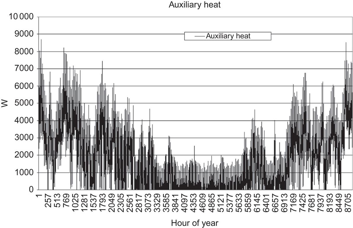
The resulting monthly average behavior is shown in Fig. 6.49, and Figs. 6.50–6.51 show the hour-by-hour behavior of storage temperature and the requirement for auxiliary heat.

Figure 6.49 Monthly simulation results for a small PVT system placed in Denmark. See discussion in text.

Figure 6.50 Hourly storage temperatures from NSES simulation of a small PVT system.

Figure 6.51 Hourly auxiliary heat requirements from NSES simulation of a small PVT system.

The top two panels in Fig. 6.49 show the monthly collection of heat and electricity and compare it with demands. The heat diagram also shows the indirect heat gains from persons, activities, and windows and the auxiliary heat needed in order to cover the total hot water and heating needs. Evidently, the solar system contributes little heat or electricity during winter months. During summer, solar electricity production is still far below building demands, whereas solar heat production covers up to two-thirds of demands. Percentages relative to loads are shown in the middle line of panels; for heat, percentages relative to the load remaining after application of auxiliary heat input are also shown.

The bottom line of diagrams shows the average temperatures of the water tank and of the ambient air and the efficiencies of electric and thermal conversion, plus first and second law thermodynamic efficiencies. The electric efficiency deviates a little from 15% in a downward direction, due to the thermal effect during summer months. The thermal efficiency remains >40% year-round; the first law efficiency is the sum of electric and thermal efficiencies; and the second law efficiency is only slightly greater than the electric efficiency, due to the modest temperature rises accomplished by the solar system.

The simulated hourly course of storage temperatures given in Fig. 6.50 shows that the solar system contributes to space heating during the period from April through September (storage temperature above 28°C). The store temperature rarely exceeds 50°C, so some auxiliary energy is needed for hot water year-round, as is shown in Fig. 6.49. This could be partially avoided by lowering the flow rate of the water passed through the collector circuit, with some associated decrease in thermal efficiency. Figure 6.51 gives the temporal distribution of auxiliary heat added in order to cover the demand at all times; there are some days even in winter where the system is able to cover the space heating need.

6.5.1.6 Medium-size PVT system simulation

The medium system considered has 6 m² of PVT collectors, but still a very modest heat store (200 liters), because long-term storage is not intended, given the collector size, solar radiation conditions at the location (Denmark), and load. As the middle left entry in Fig. 6.53 indicates, it is now possible to cover >30% of the electricity load during the months of May, June, and July. Also for heat, the coverage in summer is high (roughly 100% in July), due to the higher summer storage temperature (see Fig. 6.55) relative to the small system considered in the previous subsection. From May to October 1, the storage temperature oscillates between 15°C and 80°C.

The 15% electricity production makes the heat-collection efficiency (bottom line, Fig. 6.53) almost constantly 15% below that of a pure thermal system of the same size, the monthly simulation results of which are shown in Fig. 6.52. During summer, the system without electricity production has a higher average store temperature (in July, 60°C as compared to 50°C), whereas during winter months there is no difference. The thermal efficiency of the PVT system is, on average, 35%, with small variations: during spring and autumn, 40% is reached, whereas during the summer, a minimum of 30% coincides with the peak store temperature.

Figure 6.52 Monthly simulation results for a medium-size, pure thermal solar system.

Figure 6.53 Monthly simulation results for a medium-size PVT system. See discussion in text.

Figure 6.54 shows the solar thermal gain for each hour of the year and the energy gain by the heat store, which is a little less, due to incomplete transfer through the heat exchangers (solar absorber to working fluid and working fluid to store). Figure 6.55 gives the hourly store temperatures, which are more appropriate for the heating applications than those of the small system considered in Fig. 6.50. As a consequence, the need for auxiliary heat, shown in Fig. 6.57, is reduced, particularly during the summer. Figure 6.56 shows the net heat drawn from the store to the load circuits (hot water and air duct heating), including heat losses through the store insulation. During winter, the net heat drawn is seen to be often negative. This is when auxiliary energy is used to satisfy the load. The auxiliary energy brings the amount of hot water needed up to the required temperature and likewise the amount of air circulated between the heat store and load areas. The return air and water (after the load heat exchange) may in winter have temperatures above that of the store and thus actually help to increase the store temperature. The implied “net solar gain to store” is therefore negative, as non-solar heat is used to heat the store.

Figure 6.54 Hourly solar heat gains from simulation of a medium-size PVT system.

Figure 6.55 Hourly storage temperatures from simulation of a medium-size PVT system.

Figure 6.56 Net heat drawn hourly from store from simulation of a medium-size PVT system.

Figure 6.57 Hourly auxiliary heat requirements from simulation of a medium-size PVT system.

6.5.1.7 Large PVT system simulation

The large system considered has 40 m² of PVT collectors and 40 m³ of water storage. This may be divided into two hemispherical parts with a common interface, to simulate stratification. The input to the collector is from the lower store, and the heat to load is extracted from the upper part, provided it has a temperature higher than the lower one. The water passing through the solar collector is delivered at the top of the upper store, where a heat-exchanger spiral is continuing down to the lower store. This means that if the temperature of the water heated by the solar collector exceeds that of the upper store, it delivers energy to that store and reaches the lower store at a diminished temperature, possibly allowing it to pass further heat to the lower part. This is not meant as a substitute for a more detailed simulation of stratification, which is not done here.

The input parameters are as in Table 6.8, but with two storage compartments of 20 m³ of water and heat-loss coefficients (U-values) of 0.55. The heat loss from the stores is diminished to about a tenth of the value that would be proper for a single store with 20–30 cm of insulation, because it is supposed that some 100 buildings share a common store, in which case the surface-to-volume advantage allows this kind of reduction (cf. the simulations made in Sørensen, 1979, the first edition of this book). The program has been instructed to perform a 1% mixing of the upper and lower store for each iteration step (here 1 h), as a crude model of the stratification of a single storage volume. The resulting average store temperatures are indicated in the lower line of Fig. 6.58 and in more detail in Fig. 6.60. It is seen that the mixing does not allow temperature differences between top and bottom to persist for very long.

Figure 6.58 Monthly NSES simulation results for a large PVT system. See text for details.

Figure 6.59 Hourly solar gains from simulation of a large PVT system.

Figure 6.60 Hourly storage temperatures for NSES simulation of a large PVT system.

The top diagrams of Fig. 6.58 show that electricity needs are covered from late March to early September, but that solar heat is only able to satisfy demand without assistance from late March to the end of August. There is a strong asymmetry between the behavior in spring and autumn, which is directly caused by the temperature variations of the store and thus the collector circuit inlet temperature. The store temperature remains high until November, which causes the thermal solar collection to perform poorly, while, on the other hand, the store is capable of satisfying heat demands from heat collected earlier, as shown in the middle, right-hand diagram: there is no need for auxiliary heat from May to November. This proves that the store is large enough to act as a seasonal store, but, on the other hand, there is a very negative effect on solar thermal collection during the later months of the year. This is borne out very clearly by the efficiency curves on the lower right.

The hourly solar gain shown in Fig. 6.59 supports this interpretation, showing a clear asymmetry between spring and autumn, with a very poor performance toward the end of the year. The hourly course of storage temperature (1 is lower store, 2 is upper) is shown in Fig. 6.60. It peaks in August and has its minimum value in February; that is, it is displaced by 1–2 months relative to the solar radiation. Due to the size of the store, there are no rapid variations like those for the store temperature of the smaller systems shown in Figs. 6.50 and 6.55.

The net heat drawn from the (two) stores is given in Fig. 6.61. The negative values explained above are now confined to a few weeks in January and February. Finally, Fig. 6.62 gives the necessary auxiliary heat inputs, which are still substantial during winter, although the solar heating system now satisfies all loads from May to November.

Figure 6.61 Net heat drawn hourly from the two stores of the large PVT system.

Figure 6.62 Hourly auxiliary heat requirements for the large PVT system.

6.5.1.8 PVT Systems with heat pump

The final set of calculations adds a heat pump operating in mode 3 (see the discussion associated with Fig. 6.47) to the large PVT system. In mode 3, the heat pump operates on the heat store as its lower temperature reservoir and delivers heat at appropriate temperatures for covering space heating and hot water needs. Setting the control temperature of the heat pump to 50°C, it is possible to deliver all auxiliary heat from the heat-pump system. The monthly system performance curves are shown in Fig. 6.63. In the electricity diagram (upper right), the electric energy inputs to the heat pump are indicated. At the peak, they increase the electricity demand by nearly 70%.

Figure 6.63 Monthly simulation results for the large PVT system with heat pump operating in mode 3 and with control temperature 50°C (see text for details).

The store temperature curves (lower left) show that during February and March the heat pump cools the store down to a temperature below the ambient one. As a consequence, the apparent total efficiency (lower right) exceeds 100%, because heat from the surroundings is drawn into the heat store. Figure 6.64 shows how the net energy drawn from the store is now always positive, and, in order to make the distinction between hot water and space heating coverage easier, the space heating demand is shown separately in Fig. 6.65.

Figure 6.64 Net heat drawn hourly from stores for a large PVT system with heat pump operating in mode 3 and with control temperature 50°C. No other auxiliary heat is needed.

Figure 6.65 Hourly space heating demand (used for all simulation cases).

The store temperatures below 0°C are not quite realistic, partly because a water store has been assumed, so that large quantities of antifreeze additives are required (in addition to the small amounts used for the fluid in the collector circuit, due to occasional operation of the collector in situations of solar radiation and low temperatures), and partly because having a large cold store may increase the need for electric energy to the heat pump (if the store is within the building) or it may make district heating transmission more difficult (frost in pumps, etc.).

For these reasons, an alternative heat-pump run is made, where the control temperature is set at 29°C. This means that the heat pump will take care of all auxiliary energy for space heating, but not for hot water. The summary results are shown in Fig. 6.66. The store temperature now stays above 7°C (also in the detailed hourly output), and there is no longer any anomaly in the efficiency curves. The figure shows (in the upper right diagram) that the electric energy to the heat pump now is modest, but (in the upper left diagram) that some direct auxiliary heat has to be provided during winter months.

Figure 6.66 Monthly NSES simulation results for a large PVT system with heat pump operating in mode 3 and with control temperature 29°C (see text for details).

6.5.2 Wind electricity systems

Figures 6.67 and 6.68 give the variation in wind-power production for a large portion of the currently installed wind turbines in Denmark. Such data can be used for system simulation and inquiry into questions of surplus and deficit management through import/export or through storage. It is seen that, for turbines on land, maximum output peaks over four times the average are found during winter months, whereas for offshore plants, the maximum is only 2.3 times the average. This may indicate greater resource stability over water, and it may be that the power curve of the turbines used offshore is not approximating the power curve leading to maximum annual production as well as the power curve for turbines used on land. This design choice is illustrated in Fig. 6.70. Figure 6.69 shows the power duration curves for wind turbines placed on land and offshore in Denmark, as well as a combined curve for the onshore/offshore mix of a particular scenario for future wind coverage (Sørensen et al., 2001). The latter is seen to produce power during every hour of the year.

Figure 6.67 Hourly variation in wind-power production during the year 2000 for some 3000 Danish wind turbines placed on land. The overall annual average power output is normalized to one (Ravn, 2001; Eltra/Elkraft, 2001).

Figure 6.68 Hourly variation in wind-power production during the year 2000, normalized to annual average, for about 100 Danish wind turbines placed offshore (Ravn, 2001; Eltra/Elkraft, 2001).

Figure 6.69 Power duration curves for wind-power produced at a single site on land or offshore in Denmark and for a combined scenario for future generation on many sites, with substantial expansion of the offshore wind contribution, but use of only onshore sites already hosting a wind turbine today (Sørensen *et al*., 2001).

Figure 6.70 Power coefficients (percent of power in the wind) are given as a function of wind speed for four typical designs of wind energy generators (cf. Fig. 4.17), with the corresponding power output (*below*). The 1961 average power production at Risø, Denmark (height 56 m) is given in square brackets for each type of design (Sørensen, 1978a).

An example of how the power distribution of a propeller-type wind energy converter depends on design is shown in Fig. 6.70. The highest annual power production is obtained with design (a) and not design (c), which peaks at an average wind speed of 10 m s⁻¹, due to the asymmetry of the curves. The assumed hub height is 56 m, and 1961 data from Risø are used (cf. Fig. 3.34). Several of the calculations described in this section (taken from Sørensen 1976b, 1977, 1978a,b) use these data and agree remarkably with newer results, notably because hub heights of 50–60 m are the actual standard for present-day commercial wind turbines.

6.5.2.1 Wind-power system without energy storage

Power duration curves (or “time duration curves for power”) can be constructed using detailed hour-by-hour simulation, or even without it, provided that the wind-speed data exist in the form of a frequency distribution (such as the dashed curves in Fig. 3.38). Once a storage facility or an auxiliary conversion system has to be operated together with wind energy converters, the system simulation requires the retention of the time sequences of the meteorological data.

For a system without energy storage, there may be an advantage in choosing a power coefficient curve that peaks well below the peak of the frequency distribution of the power in the wind, rather than just maximizing annual production.

Figures 6.69 and 6.71 give examples of power duration curves that illustrate the advantage of dispersing the locations of turbines. In Fig. 6.69, the substantial smoothing obtained for the Danish sites currently in use, supplemented with continued build-up at offshore locations, is seen to significantly stretch the power duration curve. A similar conclusion can be drawn from Fig. 6.71, in this case for 18 locations in Denmark, Ireland, and Germany. If the wind-speed frequency distribution function is denoted h(u)=df(u)/du, where u is the scalar wind speed and f(u) is the accumulated frequency of wind speeds less than or equal to u, then the average power production is given by

$E = \int \frac{1}{2} ρ C_{p} (u) u^{3} h (u) d u$ $E = \int \frac{1}{2} ρ C_{p} (u) u^{3} h (u) d u$ (6.3)

(6.3)

for a wind energy converter with sufficient yawing capability to make the cos θ factor in (3.26) insignificantly different from unity during all (or nearly all) the time covered by the integral in (6.3). The power duration curve is then

$F (E) = \int δ (\frac{1}{2} ρ C_{p} (u) u^{3} \geq E) h (u) d u,$ $F (E) = \int δ (\frac{1}{2} ρ C_{p} (u) u^{3} \geq E) h (u) d u,$ (6.4)

(6.4)

where the δ function is unity if the inequality in its argument is fulfilled, and zero otherwise. If the data are in the form of a time-series, the integration may be made directly over dt (t is then time, in units of the total interval being integrated over) rather than over h(u)du. F(E) gives the fraction of time [i.e., of the time period being integrated over in (6.4)], during which the power generation from the wind energy converter exceeds the value E.

Figure 6.71 Annual power duration curves for wind energy systems with converters at 1, 3, or 18 different sites, based on 1973 data from West German weather stations, taken at the height 10 m but extrapolated to 72 m. The assumed power coefficient curve is similar to type (b) in Fig. 6.70. Based on Molly (1977).

The coupling of just three units, at different locations in Germany (typical distances about 240 km), is seen in Fig. 6.71 to imply practically as much improvement as the coupling of 18 units. The reason is that the maximum distances within Germany are still not sufficient to involve the frequent occurrence of entirely different wind regimes within the area, and thus the general meteorological conditions are often the same for all the converters except for minor differences, which can be taken advantage of by selecting three different locations. In order to take advantage of more different meteorological front system patterns, distances of 1000 km or more are required. A study of the synergy of 60 European sites made by Giebel (1999) still finds variations in wind-power production substantially at variance with demand, indicating a fundamental need for back-up or storage.

6.5.2.2 Regulation of a fuel-based back-up system

Consider now an existing fuel-based electricity-producing system, to which a number of wind energy converters are added with the purpose of saving fuel. It is conceivable that this will increase the requirements for regulation of the fuel-based units and lead to an increased number of starts and stops for the fuel-based units. Since most of these units will not be able to start delivering power to the grid at short notice, the decision to initiate the start-up procedure for a given unit must be taken some time in advance, based on expectations concerning the load and the fraction of load that the wind energy converters may be able to cover.

The time required for start-up of a conventional fuel-based unit is associated with preheating the boiler and turbine materials and thus depends on the time elapsed since the last usage. Traditionally, for start-up times less than 7 h, the start is called a “warm start.” Start-up times are generally diminishing due to new technology, so variations between plants of different age is often large, with old ones having start-up times of 20–60 min for coal-fired base and intermediate-load units, 1–7 h for pressurized-water fission reactors, and 5–6 h for boiling-water fission reactors (Nordel (Nordic Electricity Supply Undertakings), 1975). For fission reactors, “warm starts” assume start from an under-critical reactor with control rods in, and operating pressure. If the fuel-based units have cooled completely since the last usage, start-up times used to be 0.6–6 h for large coal plants, 18 h for a pressurized-water reactor, and 14 h (to reach 90% of the rated power) to 48 h (full power) for a boiling-water reactor. Modern coal-based plants using injection of pulverized coal dust have considerably lower start-up times, and many current power systems have been augmented by natural gas fired turbines with very short start-up times.

Now the question is to what extent the power production of the wind energy converters can be predicted in advance by time intervals corresponding to the different start-up times for the relevant fuel-based units. Two types of prediction may be considered, one being actual forecasts based on (mental or mathematical) models of the dynamics of general circulation and the other being associated with analysis of the statistical behavior of wind patterns, possibly including correlations that make simple methods of extrapolation permissible.

Standard meteorological forecasting, as practiced routinely by meteorological services throughout the world, may be very useful in predicting storms and thus in identifying periods of very high wind-power production, with advance notice usually the same as that required by the quoted start-up times for fuel-based units. However, forecasts at present are usually unable to specify very precisely the expected wind speed, if this is in the critical range of 5–10 m s⁻¹ covering the very steep part of the converter performance curve from zero to quite high production (cf. Fig. 6.70).

Therefore, it may be worth taking advantage of the correlations present in sequences of wind production data and in wind-speed data, such as those implied by the spectral decomposition (see, for example, Fig. 3.37). The continuity of the general circulation and the nature of the equations describing the atmospheric motion (section 2.3.1) combine to produce sequences of wind energy production figures that exhibit regularities of seasonal and diurnal scale as well as regularities of 3–5 days’ duration, associated with the passage of mesoscale front systems over a given geographical location. The following sections describe models based on trend extrapolation of power production sequences, models adding elements of stochastic fluctuations, and models using physical forecasting based on climate modeling.

Simple extrapolation model

Figure 6.72 shows a sequence of hourly, sequential production data for a wind energy converter [power coefficient (a) in Fig. 6.70] placed at the Risø turbine test site 56 m above the ground. After a period of insufficient wind (insufficient to start the wind energy converter), the average production rises, goes through a peak, and decreases again in a matter of about 4 days. It then follows a period of small and fluctuating production. Also, during the 4 days of large production, hourly fluctuations are superimposed on the general trend. However, it is evident that a power prediction simply saying that the production will be high, modest, or near zero on a given day, if the power production is high, modest, or low, respectively, on the previous day, will be correct quite often, and, similarly, the production during a given hour is strongly correlated with the production for the previous hour.

Figure 6.72 Hourly output from wind energy system without (*top*) and with short-term storage (*bottom*) for a 10-day period in January 1961. The wind energy converters are assumed to be of type (a) (Fig. 6.70), 56 m Risø data are used, and the 24 h energy storage is assumed to be loss-free and operated in a base-load mode (Sørensen, 1978a).

An extrapolation model may then be tried that bases the decision to initiate start-up procedures for fuel-based units on some (possibly weighted) average of the known wind energy production data for the time period immediately before.

For simplicity, the fuel-based supply system is assumed to consist of a number of identical units, each with a maximum power generation that is a tenth of the average load, E_av, for the entire grid of the utility system considered. It is assumed that the units can be regulated down to a third of their rated power, and that some are operated as base-load plants (i.e., at maximum power whenever possible), while others are operated as intermediate-load plants (i.e., at most times allowing for regulation in both upward and downward direction). The start-up time for the base-load units is assumed to be 6 h, and, once such a unit has been started, it will not be stopped for at least 24 h. The start-up time assumed for the intermediate-load units is 1 h. For simplicity, the load is factorized in the form

$E_{l o a d} = E_{a v} C_{1} C_{2},$ $E_{l o a d} = E_{a v} C_{1} C_{2},$ (6.5)

(6.5)

where E_av is the annual average load, C₁ is the seasonally varying monthly averages (such as those shown in Fig. 6.13), and C₂ is the average diurnal variations (such as those shown in Fig. 6.15). Both C₁ and C₂ are normalized so that the annual average implied by (6.5) is E_av. The approximation involved in (6.5) implies neglect of seasonal variations in diurnal load profiles, as well as weekday/holiday differences, and is used only for the purpose of illustration. The actual hourly data are used in the forecasting subsection below.

In the first set of calculations to be discussed, the extrapolation of wind-power production is based on two averages of past production. One is the average production of the preceding 24 h, A₂₄, which is used once every 24 h in conjunction with the minimum value of the expected load (6.5) for the following day to decide on the number n_base of base-load fuel-fired units to start. If this number is different from the number already in use, the change will become effective 6 h after the decision is made, according to the assumed base-load start-up time. Thus,

$n_{b a s e} = [\frac{E_{a v} C_{1} \min (C_{2}) - A_{24}}{0.1 E_{a v}}],$ $n_{b a s e} = [\frac{E_{a v} C_{1} \min (C_{2}) - A_{24}}{0.1 E_{a v}}],$

..................Content has been hidden....................

You can't read the all page of ebook, please click here login for view all page.

Table of Contents for 6.4 Implementation issues

Create new playlist

Sign In

Sign Up

6.3.4 Biofuel production

6.4 Implementation issues

6.4.1 System choice and optimization

6.4.2 Consistency of simulation

6.5 Local systems

6.5.1 Solar heat or heat-and-electricity systems

6.5.1.1 Model description

Solar radiation data used

6.5.1.2 Heat load of an individual house

6.5.1.3 Heat-pump systems

6.5.1.4 Software validation and results of simulations

6.5.1.5 Small PVT system simulation

6.5.1.6 Medium-size PVT system simulation

6.5.1.7 Large PVT system simulation

6.5.1.8 PVT Systems with heat pump

6.5.2 Wind electricity systems

6.5.2.1 Wind-power system without energy storage

6.5.2.2 Regulation of a fuel-based back-up system

Simple extrapolation model

Table of Contents for
6.4 Implementation issues