
![]()
Aggregations and Windowing
In this chapter, we will look at several of the built-in functions that are frequently used when querying data for reporting purposes. We’ll start off with the aggregate functions in their nonwindowed form. We’ll then explore the windowing functions: aggregate functions, ranking functions, analytic functions, and the NEXT VALUE FOR sequence generation function.
Aggregate functions are used to perform a calculation on one or more values, resulting in a single value. If your query has any columns with any nonwindowed aggregate functions, then a GROUP BY clause is required for the query. Table 7-1 shows the various aggregate functions.
Table 7-1. Aggregate Functions
| Function Name | Description | |
|---|---|---|
| AVG | The AVG aggregate function calculates the average of non-NULL values in a group. | |
| CHECKSUM_AGG | The CHECKSUM_AGG function returns a checksum value based on a group of rows, allowing you to potentially track changes to a table. For example, adding a new row or changing the value of a column that is being aggregated will usually result in a new checksum integer value. The reason I say “usually” is because there is a possibility that the checksum value does not change even if values are modified. | |
| COUNT | The COUNT aggregate function returns an integer data type showing the count of rows in a group, including rows with NULL values. | |
| COUNT_BIG | The COUNT_BIG aggregate function returns a bigint data type showing the count of rows in a group, including rows with NULL values. | |
| GROUPING | The GROUPING function returns 1 (True) or 0 (False) depending on whether a NULL value is due to a CUBE, ROLLUP, or GROUPING SETS operation. If False, the column expression NULL value is from the natural data. See Recipe 5-8 for usage of this function. | |
| MAX | The MAX aggregate function returns the highest value in a set of non-NULL values. | |
| MIN | The MIN aggregate function returns the lowest value in a group of non-NULL values. | |
| STDEV | The STDEV function returns the standard deviation of all values provided in the expression based on a sample of the data population. | |
| STDEVP | The STDEVP function also returns the standard deviation for all values in the provided expression, based upon the entire data population. | |
| SUM | The SUM aggregate function returns the summation of all non-NULL values in an expression. | |
| VAR | The VAR function returns the statistical variance of values in an expression based upon a sample of the provided population. | |
| VARP | The VARP function returns the statistical variance of values in an expression based upon the entire data population. | |
With the exception of the COUNT, COUNT_BIG, and GROUPING functions, all of the aggregate functions have the same syntax (the syntax and usage of the GROUPING function is discussed in Recipe 5-8; the syntax for the COUNT and COUNT_BIG functions is discussed in Recipe 7-2).
function_name ( { [ [ ALL | DISTINCT ] expression ] } )
where expression is typically the column or calculation that the function will be calculated over. If the optional keyword DISTINCT is used, then only distinct values will be considered. If the optional keyword ALL is used, then all values will be considered. If neither is specified, then ALL is used by default. Aggregate functions and subqueries are not allowed for the expression parameter.
The next few recipes demonstrate these aggregate functions.
Problem
You want to see the average rating of your products.
Solution
Use the AVG function to determine an average.
SELECT ProductID,
       AVG(Rating) AS AvgRating
FROM   Production.ProductReview
GROUP  BY ProductID;
This query produces the following result set:
ProductID     AvgRating
---------     ---------
709           5
798           5
937           3
How It Works
The AVG aggregate function calculates the average of non-NULL values in a group. To demonstrate the use of DISTINCT, let’s compare the columns returned from the following query:
SELECT StudentId,
       AVG(Grade) AS AvgGrade,
       AVG(DISTINCT Grade) AS AvgDistinctGrade
FROM  (VALUES (1, 100),
              (1, 100),
              (1, 100),
              (1, 99),
              (1, 99),
              (1, 98),
              (1, 98),
              (1, 95),
              (1, 95),
              (1, 95)
       ) dt (StudentId, Grade)
GROUP BY StudentID;
This query produces the following result set:
StudentId     AvgGrade     AvgDistinctGrade
---------     --------     ----------------
1             97           98
In this example, we have a student with 10 grades. The average of all 10 grades is 97. Within these 10 grades are 4 distinct grades. The average of these distinct grades is 98.
When utilizing the AVG function, the expression parameter must be one of the numeric data types.
7-2. Counting the Rows in a Group
Problem
You want to see the number of products you have in inventory on each shelf for your first five shelves.
Solution
Utilize the COUNT or COUNT_BIG function to return the count of rows in a group.
SELECT TOP (5)
       Shelf,
       COUNT(ProductID) AS ProductCount,
       COUNT_BIG(ProductID) AS ProductCountBig
FROM   Production.ProductInventory
GROUP  BY Shelf
ORDER  BY Shelf;
This query returns the following result set:
Shelf     ProductCount     ProductCountBig
-----     ------------     ---------------
A         81               81
B         36               36
C         55               55
D         50               50
E         85               85
How It Works
The COUNT and COUNT_BIG functions are utilized to return a count of the number of items in a group. The only difference between them is the data type returned: COUNT returns an INTEGER, while COUNT_BIG returns a BIGINT. The syntax for these functions is as follows:
COUNT | COUNT_BIG ( { [ [ ALL | DISTINCT ] expression ] | * } )
The difference between this syntax and the other aggregate functions is the optional asterisk (*) that can be specified. When COUNT(*) is utilized, this specifies that all rows should be counted to return the total number of rows within a table without getting rid of duplicates. COUNT(*) does not use any parameters, so it does not use any information about any column.
When utilizing the COUNT or COUNT_BIG function, the expression parameter can be of any data type except for the text, image, or ntext data type.
7-3. Summing the Values in a Group
Problem
You want to see the total due by account number for orders placed.
Summary
Utilize the SUM function to add up a column.
SELECT TOP (5)
       AccountNumber,
       SUM(TotalDue) AS TotalDueByAccountNumber
FROM   Sales.SalesOrderHeader
GROUP BY AccountNumber
ORDER BY AccountNumber;
This code returns the following result set:
AccountNumber      TotalDueByAccountNumber
--------------     -----------------------
10-4020-000001     95924.0197
10-4020-000002     28309.9672
10-4020-000003     407563.0075
10-4020-000004     660645.9404
10-4020-000005     97031.2173
How It Works
The SUM function returns the total of all values in the column being totaled. If the DISTINCT keyword is specified, the total of the distinct values in the column will be returned.
When utilizing the SUM function, the expression parameter must be one of the exact or approximate numeric data types, except for the bit data type.
7-4. Finding the High and Low Values in a Group
Problem
You want to see the highest and lowest ratings given on your products.
Solution
Utilize the MAX and MIN functions to return the highest and lowest ratings.
SELECT MIN(Rating) MinRating,
       MAX(Rating) MaxRating
FROM   Production.ProductReview;
This query returns the following result set:
MinRating     MaxRating
---------     ---------
2             5
How It Works
The MAX and MIN functions return the highest and lowest values from the expression being evaluated. Since nonaggregated columns are not specified, a GROUP BY clause is not required.
When utilizing the MAX and MIN functions, the expression parameter can be of any of the numeric, character, uniqueidentifier, or datetime data types.
7-5. Detecting Changes in a Table
Problem
You need to determine whether any changes have been made to the data in a column.
Solution
Utilize the CHECKSUM_AGG function to detect changes in a table.
SELECT StudentId,
       CHECKSUM_AGG(Grade) AS GradeChecksumAgg
FROM (VALUES (1, 100),
             (1, 100),
             (1, 100),
             (1, 99),
             (1, 99),
             (1, 98),
             (1, 98),
             (1, 95),
             (1, 95),
             (1, 95)
      ) dt (StudentId, Grade)
GROUP BY StudentID;

SELECT StudentId,
       CHECKSUM_AGG(Grade) AS GradeChecksumAgg
FROM   (VALUES (1, 100),
               (1, 100),
               (1, 100),
               (1, 99),
               (1, 99),
               (1, 98),
               (1, 98),
               (1, 95),
               (1, 95),
               (1, 90)
         ) dt (StudentId, Grade)
GROUP BY StudentID;
These queries return the following result sets:
StudentId     GradeChecksumAgg
---------     ----------------
1             59

StudentId     GradeChecksumAgg
---------     ----------------
1             62
How It Works
The CHECKSUM_AGG function returns the checksum of the values in the group, in this case the Grade column. In the second query, the last grade is changed, and when the query is rerun, the aggregated checksum returns a different value.
When utilizing the CHECKSUM_AGG function, the expression parameter must be an integer data type.
![]() Note Because of the hashing algorithm being used, it is possible for the CHECKSUM_AGG function to return the same value with different data. You should use this only if your application can tolerate occasionally missing a change.
Note Because of the hashing algorithm being used, it is possible for the CHECKSUM_AGG function to return the same value with different data. You should use this only if your application can tolerate occasionally missing a change.
7-6. Finding the Statistical Variance in the Values of a Column
Problem
You need to find the statistical variance of the data values in a column.
Solution
Utilize the VAR or VARP functions to return statistical variance.
SELECT VAR(TaxAmt) AS Variance_Sample,
       VARP(TaxAmt) AS Variance_EntirePopulation
FROM   Sales.SalesOrderHeader;
This query returns the following result set:
Variance_Sample      Variance_EntirePopulation
----------------     -------------------------
1177342.57277401     1177305.15524429
How It Works
The VAR and VARP functions return the statistical variance of all the values in the specified expression. VAR returns the value based upon a sample of the data population; VARP returns the value based upon the entire data population.
When utilizing the VAR or VARP functions, the expression parameter must be one of the exact or approximate numeric data types, except for the bit data type.
7-7. Finding the Standard Deviation in the Values of a Column
Problem
You need to see the standard deviation of the data values in a column.
Solution
Utilize the STDEV and STDEVP functions to obtain standard deviation values.
SELECT STDEV(UnitPrice) AS StandDevUnitPrice,
       STDEVP(UnitPrice) AS StandDevPopUnitPrice
FROM   Sales.SalesOrderDetail;
This query returns the following result set:
StandDevUnitPrice     StandDevPopUnitPrice
-----------------     --------------------
751.885080772954      751.881981921885
How It Works
The STDEV or STDEVP functions return the standard deviation of all the values in the specified expression. STDEV returns the value based upon a sample of the data population; STDEVP returns the value based upon the entire data population.
When utilizing the STDEV or STDEVP functions, the expression parameter must be one of the exact or approximate numeric data types, except for the bit data type.
Windowing Functions
SQL Server is designed to work best on sets of data. By definition, sets of data are unordered; it is not until the final ORDER BY clause that the final results of the query become ordered. Windowing functions allow your query to look at only a subset of the rows being returned by your query to apply the function to. In doing so, they allow you to specify an order to your unordered data set before the final result is ordered. This allows for processes that previously required self-joins, use of inefficient inequality operators, or non-set-based row-by-row processing to use set-based processing.
The key to windowing functions is in controlling the order that the rows are evaluated in, when the evaluation is restarted, and what set of rows within the result set to consider for the function (the window of the data set that the function will be applied to). These actions are performed with the OVER clause.
There are four groups of functions that the OVER clause can be applied to; in other words, there are four groups of functions that can be windowed. These groups are the aggregate functions, the ranking functions, the analytic functions, and the sequence function.
The syntax for the OVER clause is as follows:
OVER (
  [ <PARTITION BY clause> ]
  [ <ORDER BY clause> ]
  [ <ROW or RANGE clause> ]
  )

<PARTITION BY clause> ::=
PARTITION BY value_expression , ... [ n ]

<ORDER BY clause> ::=
ORDER BY order_by_expression
  [ COLLATE collation_name ]
  [ ASC | DESC ]
  [ ,... n ]

<ROW or RANGE clause> ::=
{ ROWS | RANGE } <window frame extent>

<window frame extent> ::=
{ <window frame preceding>
 | <window frame between>
}

<window frame between> ::=
 BETWEEN <window frame bound> AND <window frame bound>

<window frame bound> ::=
{ <window frame preceding>
 | <window frame following>
}

<window frame preceding> ::=
{
  UNBOUNDED PRECEDING
 | <unsigned_value_specification> PRECEDING
 | CURRENT ROW
}

<window frame following> ::=
{
  UNBOUNDED FOLLOWING
 | <unsigned_value_specification> FOLLOWING
 | CURRENT ROW
}

<unsigned value specification> ::=
{ <unsigned integer literal> }
Table 7-2 explains each of these parameters.
Table 7-2. OVER Clause Parameters
Each of the functions allows for and requires various clauses of the OVER clause.
Windowed Aggregate Functions
With the exception of the GROUPING function, all of the aggregate functions can be windowed through the OVER clause. Additionally, the new ROWS | RANGE clause allows you to perform running aggregations and sliding aggregations.
Most of the recipes in the “Windowed Aggregate Functions” section utilize the following table and data:
CREATE TABLE #Transactions
    (
    AccountId INTEGER,
    TranDate DATE,
    TranAmt NUMERIC(8, 2)
    );
INSERT INTO #Transactions
SELECT *
FROM ( VALUES ( 1, '2011-01-01', 500),
              ( 1, '2011-01-15', 50),
              ( 1, '2011-01-22', 250),
              ( 1, '2011-01-24', 75),
              ( 1, '2011-01-26', 125),
              ( 1, '2011-01-28', 175),
              ( 2, '2011-01-01', 500),
              ( 2, '2011-01-15', 50),
              ( 2, '2011-01-22', 25),
              ( 2, '2011-01-23', 125),
              ( 2, '2011-01-26', 200),
              ( 2, '2011-01-29', 250),
              ( 3, '2011-01-01', 500),
              ( 3, '2011-01-15', 50 ),
              ( 3, '2011-01-22', 5000),
              ( 3, '2011-01-25', 550),
              ( 3, '2011-01-27', 95 ),
              ( 3, '2011-01-30', 2500)
    ) dt (AccountId, TranDate, TranAmt);
7-8. Calculating Totals Based Upon the Prior Row
Problem
You need to calculate the total of a column where the total is the sum of the column through the current row. For instance, for each account, calculate the total transaction amount to date in date order.
Solution
Utilize the SUM function with the OVER clause to perform a running total.
SELECT AccountId,
       TranDate,
       TranAmt,
       -- running total of all transactions
       RunTotalAmt = SUM(TranAmt) OVER (PARTITION BY AccountId ORDER BY TranDate)
FROM   #Transactions AS t
ORDER  BY AccountId,
       TranDate;
This query returns the following result set:
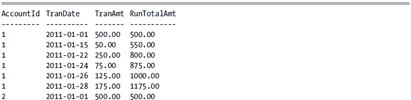
How It Works
The OVER clause, when used in conjunction with the SUM function, allows us to perform a running total of the transaction. Within the OVER clause, the PARTITION BY clause is specified to restart the calculation every time the AccountId value changes. The ORDER BY clause is specified to determine in which order the rows should be calculated. Since the ROWS | RANGE clause is not specified, the default RANGE BETWEEN UNBOUNDED PRECEDING AND CURRENT ROW is utilized. When the query is executed, the TranAmt column from all of the rows prior to and including the current row is summed up and returned.
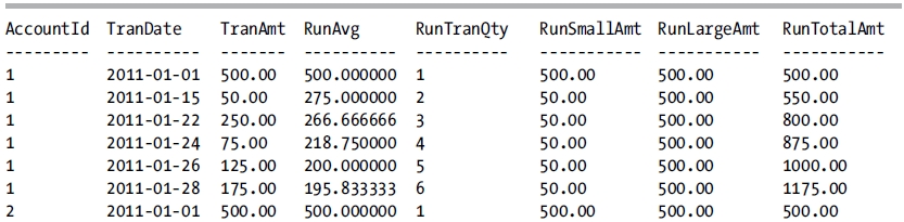
Running aggregations can be performed over the other aggregate functions also. In this next example, the query is modified to perform running averages, counts, and minimum/maximum calculations.
SELECT AccountId,
       TranDate,
       TranAmt,
       -- running average of all transactions
       RunAvg = AVG(TranAmt) OVER (PARTITION BY AccountId ORDER BY TranDate),
       -- running total # of transactions
       RunTranQty = COUNT(*) OVER (PARTITION BY AccountId ORDER BY TranDate),
       -- smallest of the transactions so far
       RunSmallAmt = MIN(TranAmt) OVER (PARTITION BY AccountId ORDER BY TranDate),
       -- largest of the transactions so far
       RunLargeAmt = MAX(TranAmt) OVER (PARTITION BY AccountId ORDER BY TranDate),
       -- running total of all transactions
       RunTotalAmt = SUM(TranAmt) OVER (PARTITION BY AccountId ORDER BY TranDate)
FROM   #Transactions AS t
ORDER BY AccountId,
         TranDate;
This query returns the following result set:
7-9. Calculating Totals Based Upon a Subset of Rows
Problem
When performing these aggregations, you want only the current row and the two previous rows to be considered for the aggregation.
Solution
Utilize the ROWS clause of the OVER clause.
SELECT AccountId,
       TranDate,
       TranAmt,
       -- average of the current and previous 2 transactions
       SlideAvg = AVG(TranAmt)
                  OVER (PARTITION BY AccountId
                            ORDER BY TranDate
                             ROWS BETWEEN 2 PRECEDING AND CURRENT ROW),
       -- total # of the current and previous 2 transactions
       SlideQty = COUNT(*)
                  OVER (PARTITION BY AccountId
                            ORDER BY TranDate
                             ROWS BETWEEN 2 PRECEDING AND CURRENT ROW),
       -- smallest of the current and previous 2 transactions
       SlideMin = MIN(TranAmt)
                  OVER (PARTITION BY AccountId
                            ORDER BY TranDate
                             ROWS BETWEEN 2 PRECEDING AND CURRENT ROW),
       -- largest of the current and previous 2 transactions
       SlideMax = MAX(TranAmt)
                  OVER (PARTITION BY AccountId
                            ORDER BY TranDate
                             ROWS BETWEEN 2 PRECEDING AND CURRENT ROW),
       -- total of the current and previous 2 transactions
       SlideTotal = SUM(TranAmt)
                  OVER (PARTITION BY AccountId
                            ORDER BY TranDate
                             ROWS BETWEEN 2 PRECEDING AND CURRENT ROW)
FROM #Transactions AS t
ORDER BY AccountId,
      TranDate;
This query returns the following result set:
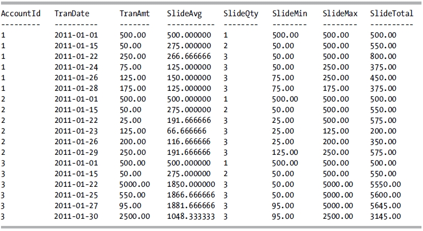
How It Works
The ROWS clause is added to the OVER clause of the aggregate functions to specify that the aggregate functions should look only at the current row and the previous two rows for their calculations. As you look at each column in the result set, you can see that the aggregation was performed over just these rows (the window of rows that the aggregation is applied to). As the query progresses through the result set, the window slides to encompass the specified rows relative to the current row.
Problem
You want the rows being considered by the OVER clause to be affected by the value in the column instead of the physical ordering.
Solution
In the OVER clause, utilize the RANGE clause instead of the ROWS option.
DECLARE @Test TABLE
        (
        RowID INT IDENTITY,
        FName VARCHAR(20),
        Salary SMALLINT
        );

INSERT INTO @Test (FName, Salary)
VALUES ('George', 800),
       ('Sam', 950),
       ('Diane', 1100),
       ('Nicholas', 1250),
       ('Samuel', 1250),
       ('Patricia', 1300),
       ('Brian', 1500),
       ('Thomas', 1600),
       ('Fran', 2450),
       ('Debbie', 2850),
       ('Mark', 2975),
       ('James', 3000),
       ('Cynthia', 3000),
       ('Christopher', 5000);

SELECT RowID,
       FName,
       Salary,
       SumByRows = SUM(Salary)
                   OVER (ORDER BY Salary
                         ROWS UNBOUNDED PRECEDING),
       SumByRange = SUM(Salary)
                    OVER (ORDER BY Salary
                         RANGE UNBOUNDED PRECEDING)
FROM @Test
ORDER BY RowID;
This query returns the following result set:
How It Works
When utilizing the RANGE clause, the SUM function adjusts its window based upon the values in the specified column. The previous example shows the salary of your employees, and the SUM function is performing a running total of the salaries in order of the salary. For comparison purposes, the running total is being calculated with both the ROWS and RANGE clauses. There are two groups of employees that have the same salary: RowIDs 4 and 5 are both 1,250, and 12 and 13 are both 3,000. When the running total is calculated with the ROWS clause, you can see that the salary of the current row is being added to the prior total of the previous rows. However, when the RANGE clause is used, all of the rows that contain the value of the current row are totaled and added to the total of the previous value. The result is that for rows 4 and 5, both employees with a salary of 1,250 are added together for the running total (and this action is repeated for rows 12 and 13).
Ranking functions allow you to return a ranking value associated to each row in a partition of a result set. Depending on the function used, multiple rows may receive the same value within the partition, and there may be gaps between assigned numbers. Table 7-3 describes the four ranking functions.
Table 7-3. Ranking Functions
| Function | Description |
|---|---|
| ROW_NUMBER | ROW_NUMBER returns an incrementing integer for each row within a partition of a set. |
| RANK | Similar to ROW_NUMBER, RANK increments its value for each row within a partition of the set. The key difference is if rows with tied values exist within the partition, they will receive the same rank value, and the next value will receive the rank value as if there had been no ties, producing a gap between assigned numbers. |
| DENSE_RANK | The difference between DENSE_RANK and RANK is that DENSE_RANK doesn’t have gaps in the rank values when there are tied values; the next value has the next rank assignment. |
| NTILE | NTILE divides the result set into a specified number of groups, based on the ordering and optional partition clause. |
The syntax of the ranking functions is as follows:
ROW_NUMBER ( ) | RANK ( ) | DENSE_RANK ( ) | NTILE (integer_expression)
  OVER ( [ PARTITION BY value_expression , ... [ n ] ] order_by_clause )
where the optional PARTITION BY clause is a list of columns that control when to restart the numbering. If the PARTITION BY clause isn’t specified, all of the rows in the result set are treated as one partition. The ORDER BY clause determines the order in which the rows within a partition are assigned their unique row number value. For the NTILE function, the integer_expression is a positive integer constant expression.
7-11. Generating an Incrementing Row Number
Problem
You need to have a query return total sales information. You need to assign a row number to each row in order of the date of the order, and the numbering needs to start over for each account number.
Solution
Utilize the ROW_NUMBER function to assign row numbers to each row.
SELECT TOP 10
       AccountNumber,
       OrderDate,
       TotalDue,
       ROW_NUMBER() OVER (PARTITION BY AccountNumber ORDER BY OrderDate) AS RN
FROM Sales.SalesOrderHeader
ORDER BY AccountNumber;
This query returns the following result set:
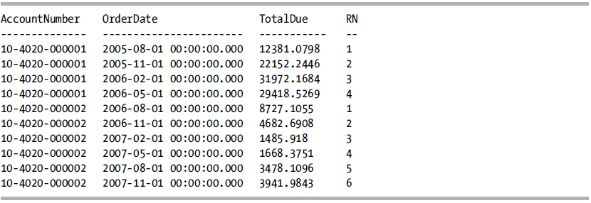
How It Works
The ROW_NUMBER function is utilized to generate a row number for each row in the partition. The PARTITION_BY clause is utilized to restart the number generation for each change in the AccountNumber column. The ORDER_BY clause is utilized to order the numbering of the rows in the order of the OrderDate column.
You can also utilize the ROW_NUMBER function to create a virtual numbers, or tally, table.
![]() Note A numbers, or tally, table is simply a table of sequential numbers, and it can be utilized to eliminate loops. Use your favorite Internet search tool to find information about what the numbers or tally table is and how it can replace loops. One excellent article is at www.sqlservercentral.com/articles/T-SQL/62867/.
Note A numbers, or tally, table is simply a table of sequential numbers, and it can be utilized to eliminate loops. Use your favorite Internet search tool to find information about what the numbers or tally table is and how it can replace loops. One excellent article is at www.sqlservercentral.com/articles/T-SQL/62867/.
For instance, the sys.all_columns system view has more than 8,000 rows. You can utilize this to easily build a numbers table with this code:
SELECT ROW_NUMBER() OVER (ORDER BY (SELECT NULL)) AS RN
FROM sys.all_columns;
This query will produce a row number for each row in the sys.all_columns view. In this instance, the ordering doesn’t matter, but it is required, so the ORDER BY clause is specified as "(SELECT NULL)". If you need more records than what are available in this table, you can simply cross join this table to itself, which will produce more than 64 million rows.
In this example, a table scan is required. Another method is to produce the numbers or tally table by utilizing constants. The following example creates a one million row virtual tally table without incurring any disk I/O operations:
WITH
TENS      (N) AS (SELECT 0 UNION ALL SELECT 0 UNION ALL SELECT 0 UNION ALL
                  SELECT 0 UNION ALL SELECT 0 UNION ALL SELECT 0 UNION ALL
                  SELECT 0 UNION ALL SELECT 0 UNION ALL SELECT 0 UNION ALL SELECT 0),
THOUSANDS (N) AS (SELECT 1 FROM TENS t1 CROSS JOIN TENS t2 CROSS JOIN TENS t3),
MILLIONS  (N) AS (SELECT 1 FROM THOUSANDS t1 CROSS JOIN THOUSANDS t2),
TALLY     (N) AS (SELECT ROW_NUMBER() OVER (ORDER BY (SELECT 0)) FROM MILLIONS)
SELECT N
FROM TALLY;
7-12. Returning Rows by Rank
Problem
You want to rank your salespeople based upon their sales quota.
Solution
Utilize the RANK function to rank your salespeople.
SELECT BusinessEntityID,
       QuotaDate,
       SalesQuota,
       RANK() OVER (ORDER BY SalesQuota DESC) AS RANK
FROM   Sales.SalesPersonQuotaHistory
WHERE  SalesQuota BETWEEN 266000.00 AND 319000.00;
This query returns the following result set:
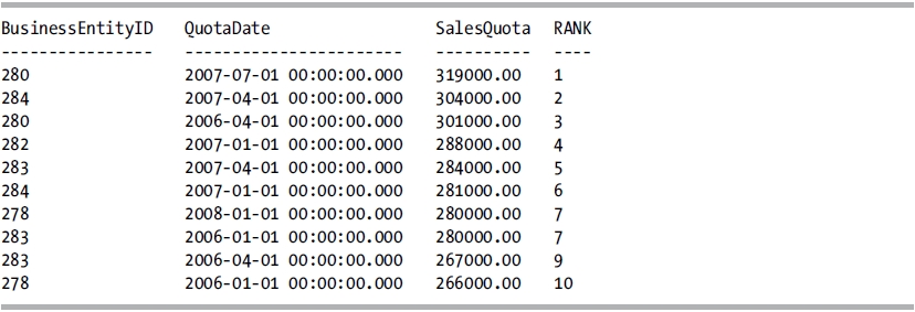
How It Works
RANK assigns a ranking value to each row within a partition. If multiple rows within the partition tie with the same value, they are assigned the same ranking value (see rank 7 in the example). When there is a tie, the following value has a ranking value assigned as if none of the previous rows had ties. If there are no ties in the partition, the ranking value assigned is the same as if the ROW_NUMBER function had been used with the same OVER clause definition.
7-13. Returning Rows by Rank Without Gaps
Problem
You want to rank your salespeople based upon their sales quota without any gaps in the ranking value assigned.
Solution
Utilize the DENSE_RANK function to rank your salespeople without gaps.
SELECT BusinessEntityID,
       QuotaDate,
       SalesQuota,
       DENSE_RANK() OVER (ORDER BY SalesQuota DESC) AS DENSERANK
FROM   Sales.SalesPersonQuotaHistory
WHERE  SalesQuota BETWEEN 266000.00 AND 319000.00;
This query returns the following result set:
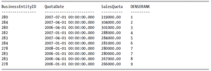
How It Works
DENSE_RANK assigns a ranking value to each row within a partition. If multiple rows within the partition tie with the same value, they are assigned the same ranking value (see rank 7 in the example). When there is a tie, the following value has the next ranking value assigned. If there are no ties in the partition, the ranking value assigned is the same as if the ROW_NUMBER function had been used with the same OVER clause definition.
7-14. Sorting Rows into Buckets
Problem
You want to split your salespeople up into four groups based upon their sales quota.
Solution
Utilize the NTILE function, and specify the number of groups to divide the result set into.
SELECT BusinessEntityID,
       QuotaDate,
       SalesQuota,
       NTILE(4) OVER (ORDER BY SalesQuota DESC) AS [NTILE]
FROM   Sales.SalesPersonQuotaHistory
WHERE  SalesQuota BETWEEN 266000.00 AND 319000.00;
This query produces the following result set:
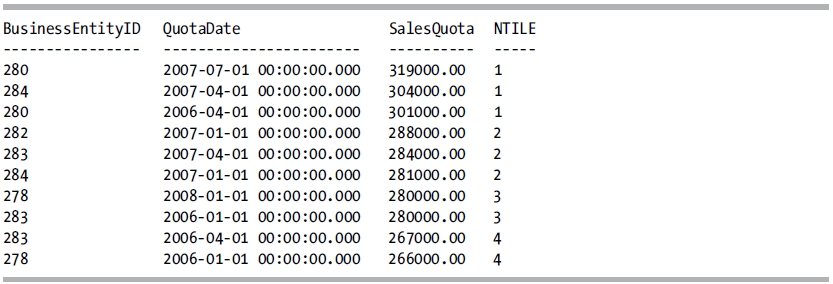
How It Works
The NTILE function divides the result set into the specified number of groups based upon the partitioning and ordering specified in the OVER clause. Notice that the first two groups have three rows in that group, and the final two groups have two. If the number of rows in the result set is not evenly divisible by the specified number of groups, then the leading groups will have one extra row assigned to that group until the remainder has been accommodated.
7-15. Grouping Logically Consecutive Rows Together
Problem
You need to group logically consecutive rows together so that subsequent calculations can treat those rows identically. For instance, your manufacturing plant utilizes RFID tags to track the movement of your products. During the manufacturing process, a product may be rejected and sent back to an earlier part of the process to be corrected. You want to track the number of trips that a tag makes to an area. However, you have multiple sensors to detect the tags in your larger areas, so multiple consecutive hits from different sensors can be entered in the system. These consecutive entries need to be considered together based upon the time in the same area and should be treated as the same trip in your results.
This recipe will utilize the following data:
DECLARE @RFID_Location TABLE (
    TagId INTEGER,
    Location VARCHAR(25),
    SensorDate DATETIME);
INSERT INTO @RFID_Location
        (TagId, Location, SensorDate)
VALUES (1, 'Room1', '2012-01-10T08:00:01'),
       (1, 'Room1', '2012-01-10T08:18:32'),
       (1, 'Room2', '2012-01-10T08:25:42'),
       (1, 'Room3', '2012-01-10T09:52:48'),
       (1, 'Room2', '2012-01-10T10:05:22'),
       (1, 'Room3', '2012-01-10T11:22:15'),
       (1, 'Room4', '2012-01-10T14:18:58'),
       (2, 'Room1', '2012-01-10T08:32:18'),
       (2, 'Room1', '2012-01-10T08:51:53'),
       (2, 'Room2', '2012-01-10T09:22:09'),
       (2, 'Room1', '2012-01-10T09:42:17'),
       (2, 'Room1', '2012-01-10T09:59:16'),
       (2, 'Room2', '2012-01-10T10:35:18'),
       (2, 'Room3', '2012-01-10T11:18:42'),
       (2, 'Room4', '2012-01-10T15:22:18'),
Solution
Utilize two ROW_NUMBER functions, differing only in that the last column in the PARTITION BY clause has an extra column. The difference between these results will group logically consecutive rows together.
WITH cte AS
(
SELECT TagId, Location, SensorDate,
       ROW_NUMBER()
       OVER (PARTITION BY TagId
                 ORDER BY SensorDate) -
       ROW_NUMBER()
       OVER (PARTITION BY TagId, Location
                 ORDER BY SensorDate) AS Grp
FROM @RFID_Location
)
SELECT TagId, Location, SensorDate, Grp,
       DENSE_RANK()
       OVER (PARTITION BY TagId, Location
                 ORDER BY Grp) AS TripNbr
FROM  cte
ORDER BY TagId, SensorDate;
This query returns the following result set:
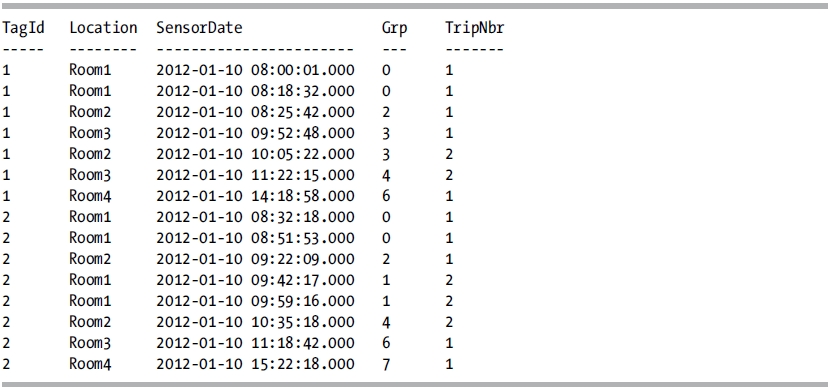
How It Works
The first ROW_NUMBER function partitions the result set by the TagId and assigns the row number as ordered by the SensorDate. The second ROW_NUMBER function partitions the result set by the TagId and Location and assigns the row number as ordered by the SensorDate. The difference between these will assign consecutive rows in the same location as the same Grp number. The previous results show that consecutive entries in the same location are assigned the same Grp number. The following query breaks the ROW_NUMBER functions down into individual columns so that you can see how this is performed:
WITH cte AS
(
SELECT TagId, Location, SensorDate,
       ROW_NUMBER()
       OVER (PARTITION BY TagId
                 ORDER BY SensorDate) AS RN1,
       ROW_NUMBER()
       OVER (PARTITION BY TagId, Location
                 ORDER BY SensorDate) AS RN2
FROM   @RFID_Location
)
SELECT TagId, Location, SensorDate,
       RN1, RN2, RN1-RN2 AS Grp
FROM   cte
ORDER BY TagId, SensorDate;
This query returns the following result set:
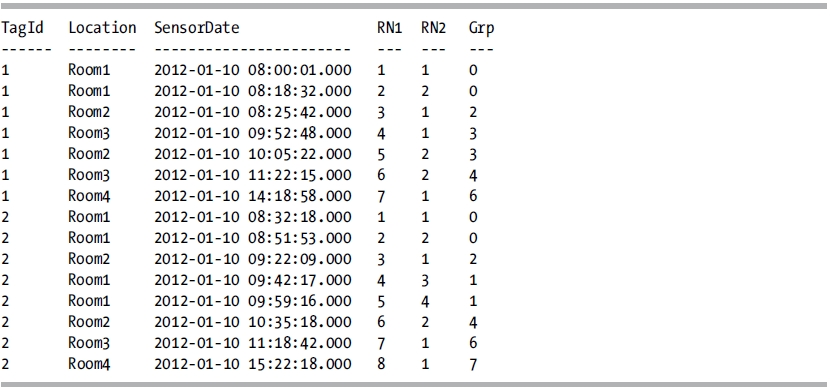
With this query, you can see that for each TagId, the RN1 column is sequentially numbered from 1 to the number of rows for that TagId. For the RN2 column, the Location is added to the PARTITION BY clause, resulting in the assigned row numbers being restarted every time the location changes. By looking at this result set, you can see that subtracting RN2 from RN1 returns a number where each trip to a location has a higher number than the previous trip, and consecutive reads in the same location are treated the same. It doesn’t matter that the calculated Grp column is not consecutive; it is the fact that it increases from the prior trip to this location that is critical. To handle calculating the trips, the DENSE_RANK function is utilized so that there will not be any gaps. The following query takes the first example and adds in the RANK function to illustrate the difference.
WITH cte AS
(
SELECT TagId, Location, SensorDate,
       ROW_NUMBER()
       OVER (PARTITION BY TagId
                 ORDER BY SensorDate) -
       ROW_NUMBER()
       OVER (PARTITION BY TagId, Location
                 ORDER BY SensorDate) AS Grp
FROM @RFID_Location
)
SELECT TagId, Location, SensorDate, Grp,
       DENSE_RANK()
       OVER (PARTITION BY TagId, Location
                 ORDER BY Grp) AS TripNbr,
       RANK()
       OVER (PARTITION BY TagId, Location
                 ORDER BY Grp) AS TripNbrRank
FROM  cte
ORDER BY TagId, SensorDate;
This query returns the following result set:
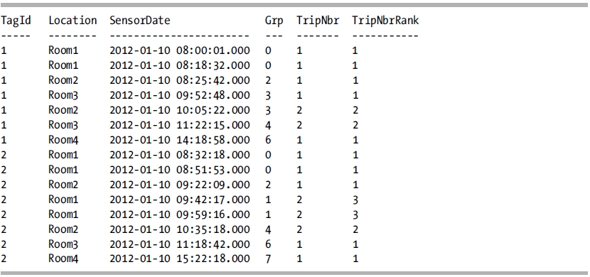
In this query, you can see how the RANK function returns the wrong trip number for TagId 2 for the second trip to Room1 (the fourth and fifth rows for this tag).
New to SQL Server 2012 are the analytic functions. Analytic functions compute an aggregate value on a group of rows. In contrast to the aggregate functions, they can return multiple rows for each group. Table 7-4 describes the analytic functions.
Table 7-4. Analytic Functions
| Function | Description |
|---|---|
| CUME_DIST | CUME_DIST calculates the cumulative distribution of a value in a group of values. The cumulative distribution is the relative position of a specified value in a group of values. |
| FIRST_VALUE | Returns the first value from an ordered set of values. |
| LAG | Retrieves data from a previous row in the same result set as specified by a row offset from the current row. |
| LAST_VALUE | Returns the last value from an ordered set of values. |
| LEAD | Retrieves data from a subsequent row in the same result set as specified by a row offset from the current row. |
| PERCENTILE_CONT | Calculates a percentile based on a continuous distribution of the column value. The value returned may or may not be equal to any of the specific values in the column. |
| PERCENTILE_DISC | Computes a specific percentile for sorted values in the result set. The value returned will be the value with the smallest CUME_DIST value (for the same sort specification) that is greater than or equal to the specified percentile. The value returned will be equal to one of the values in the specific column. |
| PERCENT_RANK | Computes the relative rank of a row within a set. |
The analytic functions come in complementary pairs and will be discussed in this manner.
7-16. Accessing Values from Other Rows
Problem
You need to write a sales summary report that shows the total due from orders by year and quarter. You want to include a difference between the current quarter and prior quarter, as well as a difference between the current quarter of this year and the same quarter of the previous year.
Solution
Aggregate the total due by year and quarter, and utilize the LAG function to look at the previous records.
WITH cte AS
(
SELECT DATEPART(QUARTER, OrderDate) AS Qtr,
       DATEPART(YEAR, OrderDate) AS Yr,
       TotalDue
FROM   Sales.SalesOrderHeader
), cteAgg AS
(
SELECT Yr,
       Qtr,
       SUM(TotalDue) AS TotalDue
FROM   cte
GROUP BY Yr, Qtr
)
SELECT Yr,
       Qtr,
       TotalDue,
       TotalDue - LAG(TotalDue, 1, NULL)
                  OVER (ORDER BY Yr, Qtr) AS DeltaPriorQtr,
       TotalDue - LAG(TotalDue, 4, NULL)
                  OVER (ORDER BY Yr, Qtr) AS DeltaPriorYrQtr
FROM cteAgg
ORDER BY Yr, Qtr;
This query returns the following result set:
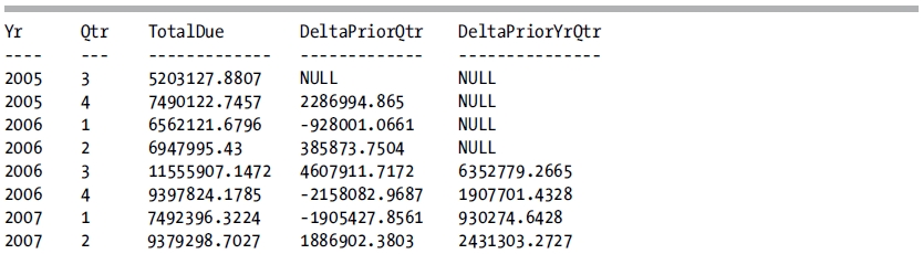
How It Works
The first CTE is utilized to retrieve the year and quarter from the OrderDate column and to pass the TotalDue column to the rest of the query. The second CTE is used to aggregate the TotalDue column, grouping on the extracted Yr and Qtr columns. The final SELECT statement returns these aggregated values and then makes two calls to the LAG function. The first call retrieves the TotalDue column from the previous row in order to compute the difference between the current quarter and the previous quarter. The second call retrieves the TotalDue column from four rows prior to the current row in order to compute the difference between the current quarter and the same quarter one year ago.
The LEAD function works in a similar manner. In this example, a table is created that has gaps in the column. The table is then queried, comparing the value in the current row to the value in the next row. If the difference is greater than 1, then a gap exists and is returned in the result set. This solution is based on a method that I learned from Itzik Ben-Gan.
DECLARE @Gaps TABLE (col1 int PRIMARY KEY CLUSTERED);

INSERT INTO @Gaps (col1)
VALUES (1), (2), (3),
       (50), (51), (52), (53), (54), (55),
       (100), (101), (102),
       (500),
       (950), (951), (952),
       (954);

-- Compare the value of the current row to the next row.
-- If > 1, then there is a gap.
WITH cte AS
(
SELECT col1 AS CurrentRow,
       LEAD(col1, 1, NULL)
       OVER (ORDER BY col1) AS NextRow
FROM   @Gaps
)
SELECT cte.CurrentRow + 1 AS [Start of Gap],
       cte.NextRow - 1 AS [End of Gap]
FROM cte
WHERE cte.NextRow - cte.CurrentRow > 1;
This query returns the following result set:
Start of Gap     End of Gap
------------     ----------
4                49
56               99
103              499
501              949
953              953
The syntax for the LAG and LEAD functions is as follows:
LAG | LEAD (scalar_expression [,offset] [,default])
  OVER ( [ partition_by_clause ] order_by_clause )
Where scalar_expression is an expression of any type that returns a scalar value (typically a column), offset is the number of rows to offset the current row by, and default is the value to return if the value returned is NULL. The default value for offset is 1, and the default value for default is NULL.
7-17. Accessing the First or Last Value from a Partition
Problem
You need to write a report that shows, for each customer, the date that they placed their least and most expensive orders.
Solution
Utilize the FIRST_VALUE and LAST_VALUE functions.
SELECT DISTINCT TOP (5)
       CustomerID,
       FIRST_VALUE(OrderDate)
       OVER (PARTITION BY CustomerID
                 ORDER BY TotalDue
                  ROWS BETWEEN UNBOUNDED PRECEDING
                          AND UNBOUNDED FOLLOWING) AS OrderDateLow,
       LAST_VALUE(OrderDate)
       OVER (PARTITION BY CustomerID
                 ORDER BY TotalDue
                  ROWS BETWEEN UNBOUNDED PRECEDING
                          AND UNBOUNDED FOLLOWING) AS OrderDateHigh
FROM   Sales.SalesOrderHeader
ORDER BY CustomerID;
This query returns the following result set for the first five customers:
| CustomerID | OrderDateLow | OrderDateHigh |
| ----------- | ----------------------- | ----------------------- |
| 11000 | 2007-07-22 00:00:00.000 | 2005-07-22 00:00:00.000 |
| 11001 | 2008-06-12 00:00:00.000 | 2005-07-18 00:00:00.000 |
| 11002 | 2007-07-04 00:00:00.000 | 2005-07-10 00:00:00.000 |
| 11003 | 2007-07-09 00:00:00.000 | 2005-07-01 00:00:00.000 |
| 11004 | 2007-07-26 00:00:00.000 | 2005-07-26 00:00:00.000 |
How It Works
The FIRST_VALUE and LAST_VALUE functions are used to return the OrderDate for the first and last rows in the partition. The window is set to a partition of the CustomerID, ordered by the TotalDue, and the ROWS clause is used to specify all of the rows for the partition (CustomerId). The syntax for the FIRST_VALUE and LAST_VALUE functions is as follows:
FIRST_VALUE ( scalar_expression )
  OVER ( [ partition_by_clause ] order_by_clause [ rows_range_clause ] )
where scalar_expression is an expression of any type that returns a scalar value (typically a column).
7-18. Calculating the Relative Position or Rank of a Value in a Set of Values
Problem
You want to know the relative position and rank of a customer’s order by the total of the order in respect to the total of all the customers’ orders.
Solution
Utilize the CUME_DIST and PERCENT_RANK functions to obtain the relative position of a value and the relative rank of a value.
SELECT CustomerID,
       CUME_DIST()
       OVER (PARTITION BY CustomerID
                 ORDER BY TotalDue) AS CumeDistOrderTotalDue,
       PERCENT_RANK()
       OVER (PARTITION BY CustomerID
                 ORDER BY TotalDue) AS PercentRankOrderTotalDue
FROM   Sales.SalesOrderHeader
ORDER BY CustomerID;
This code returns the following abridged result set:
| CustomerID | CumeDistOrderTotalDue | PercentRankOrderTotalDue |
| ---------- | --------------------- | ------------------------ |
| 30116 | 0.25 | 0 |
| 30116 | 0.5 | 0.333333333333333 |
| 30116 | 0.75 | 0.666666666666667 |
| 30116 | 1 | 1 |
| 30117 | 0.0833333333333333 | 0 |
| 30117 | 0.166666666666667 | 0.0909090909090909 |
| 30117 | 0.25 | 0.181818181818182 |
| 30117 | 0.333333333333333 | 0.272727272727273 |
| 30117 | 0.416666666666667 | 0.363636363636364 |
| 30117 | 0.5 | 0.454545454545455 |
| 30117 | 0.583333333333333 | 0.545454545454545 |
| 30117 | 0.666666666666667 | 0.636363636363636 |
| 30117 | 0.75 | 0.727272727272727 |
| 30117 | 0.833333333333333 | 0.818181818181818 |
| 30117 | 0.916666666666667 | 0.909090909090909 |
| 30117 | 1 | 1 |
| 30118 | 0.125 | 0 |
| 30118 | 0.25 | 0.142857142857143 |
| 30118 | 0.375 | 0.285714285714286 |
| 30118 | 0.5 | 0.428571428571429 |
| 30118 | 0.625 | 0.571428571428571 |
| 30118 | 0.75 | 0.714285714285714 |
| 30118 | 0.875 | 0.857142857142857 |
| 30118 | 1 | 1 |
How It Works
The CUME_DIST function returns the relative position of a value in a set of values, while the PERCENT_RANK function returns the relative rank of a value in a set of values. The syntax of these functions is as follows:
CUME_DIST() | PERCENT_RANK( )
  OVER ( [ partition_by_clause ] order_by_clause )
The result returned by these functions will be a float(53) data type, with the value being greater than 0 and less than or equal to 1 (0 < x <= 1). When utilizing these functions, NULL values will be included, and the value returned will be the lowest possible value.
7-19. Calculating Continuous or Discrete Percentiles
Problem
You want to see the median salary and the 75 percentile salary for all employees per department.
Solution
Utilize the PERCENTILE_CONT and PERCENTILE_DISC functions to return percentile calculations based upon a value at a specified percentage.
DECLARE @Employees TABLE
        (
        EmplId INT PRIMARY KEY CLUSTERED,
        DeptId INT,
        Salary NUMERIC(8, 2)
        );

INSERT INTO @Employees
VALUES (1, 1, 10000),
       (2, 1, 11000),
       (3, 1, 12000),
       (4, 2, 25000),
       (5, 2, 35000),
       (6, 2, 75000),
       (7, 2, 100000);

SELECT EmplId,
       DeptId,
       Salary,
       PERCENTILE_CONT(0.5)
        WITHIN GROUP (ORDER BY Salary ASC)
        OVER (PARTITION BY DeptId) AS MedianCont,
       PERCENTILE_DISC(0.5)
        WITHIN GROUP (ORDER BY Salary ASC)
        OVER (PARTITION BY DeptId) AS MedianDisc,
       PERCENTILE_CONT(0.75)
        WITHIN GROUP (ORDER BY Salary ASC)
        OVER (PARTITION BY DeptId) AS Percent75Cont,
       PERCENTILE_DISC(0.75)
        WITHIN GROUP (ORDER BY Salary ASC)
        OVER (PARTITION BY DeptId) AS Percent75Disc,
       CUME_DIST()
        OVER (PARTITION BY DeptId
                 ORDER BY Salary) AS CumeDist
FROM @Employees
ORDER BY DeptId, EmplId;
This query returns the following result set:

How It Works
PERCENTILE_CONT calculates a percentile based upon a continuous distribution of values of the specified column. This is performed by using the specified percentile value (SP) and the number of rows in the partition (N) and by computing the row number of interest (RN) after the ordering has been applied. The row number of interest is computed from the formula RN = (1 + (SP * (N- 1))). The result returned is the linear interpolation (essentially an average) between the values from the rows at CEILING(RN) and FLOOR(RN). The value returned may or may not exist in the partition being analyzed.
PERCENTILE_DISC calculates a percentile based upon a discrete distribution of the column values. For the specified percentile (P), the values of the partition are sorted, and the value returned will be from the row with the smallest CUME_DIST value (with the same ordering) that is greater than or equal to P. The value returned will exist in one of the rows in the partition being analyzed. Since the result for this function is based on the CUME_DIST value, that function was included in the previous query in order to show its value.
The syntax for these functions is as follows:
PERCENTILE_CONT ( numeric_literal) | PERCENTILE_DISC ( numeric_literal )
  WITHIN GROUP ( ORDER BY order_by_expression [ ASC | DESC ] )
  OVER ( [ <partition_by_clause> ] )
In the example, PERCENTILE_CONT(0.5) is utilized to obtain the median value. For DeptId = 1, there are three rows, so the median value is the value from the middle row (after sorting). For DeptId = 2, there are four rows, so the median value is the average of the two middle rows. This value does not exist in this partition.
PERCENTILE_DISC returns a value that exists in the partition, based upon the CUME_DIST value. By specifying PERCENTILE_DISC(0.5), the row in each partition that has a CUME_DIST value of .5, or the next row that is greater than .5, is utilized, and the salary for that row is returned.
Sequences are used to create an incrementing number. While similar to an identity column, they are not bound to any table, can be reset, and can be used across multiple tables. Sequences are discussed in detail in Recipe 13-22. Sequences are assigned by calling the NEXT VALUE FOR function, and multiple values can be assigned simultaneously. The order of these assignments can be controlled by use of the optional OVER clause of the NEXT VALUE FOR function.
7-20. Assigning Sequences in a Specified Order
Problem
You are inserting multiple student grades into a table. Each record needs to have a sequence assigned, and you want the sequences to be assigned in order of the grades.
Solution
Utilize the OVER clause of the NEXT VALUE FOR function, specifying the desired order.
IF EXISTS (SELECT 1
        FROM sys.sequences AS seq
        JOIN sys.schemas AS sch
        ON seq.schema_id = sch.schema_id
        WHERE sch.name = 'dbo'
        AND seq.name = 'CH7Sequence')
  DROP SEQUENCE dbo.CH7Sequence;

CREATE SEQUENCE dbo.CH7Sequence AS INTEGER START WITH 1;

DECLARE @ClassRank TABLE
        (
        StudentID TINYINT,
        Grade TINYINT,
        SeqNbr INTEGER
        );
INSERT INTO @ClassRank (StudentId, Grade, SeqNbr)
SELECT StudentId,
       Grade,
       NEXT VALUE FOR dbo.CH7Sequence OVER (ORDER BY Grade ASC)
FROM (VALUES (1, 100),
             (2, 95),
             (3, 85),
             (4, 100),
             (5, 99),
             (6, 98),
             (7, 95),
             (8, 90),
             (9, 89),
             (10, 89),
             (11, 85),
             (12, 82)) dt(StudentId, Grade);

SELECT StudentId, Grade, SeqNbr
FROM   @ClassRank;
This query returns the following result set:
| StudentID | Grade | SeqNbr |
| --------- | ----- | ------ |
| 12 | 82 | 1 |
| 3 | 85 | 2 |
| 11 | 85 | 3 |
| 10 | 89 | 4 |
| 9 | 89 | 5 |
| 8 | 90 | 6 |
| 7 | 95 | 7 |
| 2 | 95 | 8 |
| 6 | 98 | 9 |
| 5 | 99 | 10 |
| 1 | 100 | 11 |
| 4 | 100 | 12 |
How It Works
The optional OVER clause of the NEXT VALUE FOR function is utilized to specify the order that the sequence should be applied. The syntax is as follows:
NEXT VALUE FOR [ database_name . ] [ schema_name . ] sequence_name
  [ OVER (<over_order_by_clause>) ]