
Hour 14. The ggplot2 Package for Graphics
What You’ll Learn in This Hour:
![]() Creating simple plots
Creating simple plots
![]() Changing plot types
Changing plot types
![]() Control of aesthetics
Control of aesthetics
![]() Groups and panels
Groups and panels
![]() Themes and legend control
Themes and legend control
In Hour 13, “Graphics,” you saw how the graphics package can be used to create highly customized graphics. However, as you have seen, the graphics package can be hard work when used as an exploratory tool. To compare levels of a variable, we typically need to use “for” loops or a clever application of factors. Items such as the legend must be added manually.
The lattice and ggplot2 packages offer alternatives to the graphics package that are much easier to use for data exploration. Each has been built using Paul Murrell’s grid package, thus enabling plots to be created as objects that are then printed when required. In this hour we start by looking at the hugely popular ggplot2 package, developed (once again) by Hadley Wickham.
The Philosophy of ggplot2
The ggplot2 package was inspired by Leland Wilkinson’s book The Grammar of Graphics. The grammar of graphics philosophy breaks a graphic into a series of layers. Different layers describe the mapping of the data to plot features, the plot type, the coordinate system, and the associated scaling of plot features. To follow the grammar of graphic using ggplot2, we need just one plot function, ggplot, to which we add the required layers. Different plot types can be achieved through geometric layers, or “geoms.”
In addition to the relatively pure implementation of the grammar of graphics via the ggplot function, ggplot2 offers an additional graphical function, qplot, designed to speed up the creation of graphics by making assumptions about the layers we want to use. The existence of qplot in ggplot2 is divisive: Several vocal supporters of the grammar of graphics concept advocate scrapping qplot. However, as passionate ggplot2 supporters that use and teach the package on a daily basis, the authors of this book cannot relate to this opinion. Our clients want to be able to create powerful visualizations as quickly and easily as possible. Why would anyone want to remove a function that makes it quicker and easier to create high quality graphics?! By the end of the hour, you can decide for yourself whether you prefer the quick-and-easy approach, the true grammar of graphics, or a combination of the two. For now let’s take a look at some ggplot2 basics using the qplot function.
Quick Plots and Basic Control
The “q” in qplot stands for “quick.” The speed mainly relates to typing; the function requires a lot less typing than its ggplot counterpart. It achieves this by making assumptions; however, the function is also far more flexible than most people realize and can be used in conjunction with a layered grammar of graphics approach.
Using qplot
We have stated that qplot is quick because it makes assumptions. Thankfully there are very few assumptions, and they are all very sensible! Indeed, most of the assumptions are no different from the assumptions made by graphics functions such as plot and hist. In addition to assumptions about the coordinate system, axes, plotting character, and so on, qplot also makes an assumption about the plot type. For example, if we provide a single variable to qplot, it is assumed that we want to draw a histogram. If we provide two variables, it is assumed that we want to draw a scatter plot.
Later, you’ll see how to easily vary the plot type using qplot, but for now we start with a simple scatter plot using the mtcars data. We specify mtcars as the data frame that we are using and refer to the wt and mpg variables directly. The output is displayed in Figure 14.1.
> # Load package and create a simple plot
> require(ggplot2)
> theme_set(theme_bw(base_size= 14)) # Set the theme to a white background (more
later)
> qplot(x = wt, y = mpg, data = mtcars)

Tip: Changing the Default Theme
In the code block that creates Figure 14.1, we include a line to set the “theme”. This line of code changes the default background color from grey with white gridlines to white with grey gridlines. At the same time we increase the default font size. This is a global setting that changes the appearance of each of the subsequent graphics produced in this hour. We look at themes in more detail later in the hour.
Note: Working with Vectors
The qplot function allows us to directly pass individual vectors—for example, qplot(1:10, rnorm(10)). However, it is generally more common to have the data that you wish to plot stored within a data frame. In this case, it is much easier to specify the name of the data frame using the data argument so that we can refer to variables directly.
Titles and Axes
As with the plotting functions contained within the base graphics package, we can add a main title to our plot using qplot via the main argument. The arguments xlab and ylab control the axis labels for the X and Y axes, respectively. Similarly, arguments xlim and ylim allow users to control the X and Y axis limits. These arguments must be provided with a vector of length 2. We can also add these features using “layers.”
Working with Layers
To follow the grammar of graphics, we build a plot in layers. We don’t have to do this with qplot, but each of the title/axis elements that we have looked at could instead have been added using a layer. A main title as well as X and Y axis labels can also be added as layers using the ggtitle function and the xlab and ylab functions, respectively. For the X and Y axis limits, we can use xlim and ylim functions. Listing 14.1 contains two sections of code for re-creating the graphic in Figure 14.1 with an appropriate title and axis labels. The two code sections produce an identical graphic; the first, starting on line 2, uses a single call to qplot, and the second, starting on line 10, uses a layered approach.
LISTING 14.1 Optional Layering
1: > # Version 1: Using a single call to qplot
2: > qplot(x = wt, y = mpg, data = mtcars,
3: + main = "Miles per Gallon vs Weight
Automobiles (1973–74 models)",
4: + xlab = "Weight (lb/1000)",
5: + ylab = "Miles per US Gallon",
6: + xlim = c(1, 6),
7: + ylim = c(0, 40))
8: >
9: > # Version 2: qplot with additional layers
10: > qplot(x = wt, y = mpg, data = mtcars) +
11: + ggtitle("Miles per Gallon vs Weight
Automobiles (1973–74 models)") +
12: + xlab("Weight (lb/1000)") +
13: + ylab("Miles per US Gallon") +
14: + xlim(c(1, 6)) +
15: + ylim(c(0, 40))
To add plots as layers, we use the “+” symbol. By placing a + at the end of the line, we tell R to expect more layers to our plot, much like adding numbers. When we add ggplot2 functions in this way, we say we are adding “layers.”
Tip: Fixing One End of an Axis
Sometimes we’re only interested in fixing one end of an axis scale. For example, we may wish to fix the lower end at zero. In this case, NA can be used to specify that we are happy to let ggplot2 choose a bound for us.
Plots as Objects
Both lattice and ggplot2 are built using Paul Murrell’s grid package. This allows us to save plots as objects. The qplot function creates a ggplot object. A ggplot object is essentially a set of instructions that explain how to create the graphic. Only when we ask R to print the object are the instructions followed and the graph created. The instructions can be saved and used at any time—for example, after we have altered some theme settings and we are ready to export our graphics.
> # Create a basic plot and save it as an object
> basicCarPlot <- qplot(wt, mpg, data = mtcars)
> # Modify the plot to include a title
> basicCarPlot <- basicCarPlot +
+ ggtitle("Miles per Gallon vs Weight
Automobiles (1973–74 models)")
> # Now print the plot
> basicCarPlot
We can use layers to modify a ggplot object, adding new instructions as to what to draw. This is extremely powerful for data exploration because it allows us to create a base graphic and use a variety of different additional layers to explore covariates.
Tip: Exporting ggplot2 Graphics
In Hour 13 you saw how to write a plot to file by opening the device, drawing the plot, and then closing the device with dev.off. The ggplot2 package provides an alternative workflow via ggsave. To export using ggsave, we first save our plot as an object. When we are ready to write the plot to file, we pass ggsave the filename and ggplot the object name, for example:
> carPlot <- qplot(x = wt, y = mpg, data = mtcars) # Create ggplot object
> ggsave(file = "carPlot.png", carPlot) # Save object as a png
Saving 10.6 x 7.57 in image
The function handles the opening and closing of devices for us, selecting the device based on the file extension that we provide.
Changing Plot Types
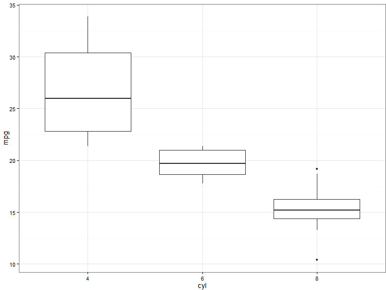
Using the grammar of graphics terminology, plot types are considered to be geometric shapes that describe how the data are displayed. We vary the plot type using the geom (short for “geometric”) argument to qplot, negating the need for separate plotting functions. A sample call is shown here with the resulting graphic shown in Figure 14.2:
> # Ensure cyl variable is of the right type by fixing in the data
> mtcars$cyl <- factor(mtcars$cyl)
> qplot(cyl, mpg, data = mtcars, geom = "boxplot")
Caution: Know Your Factors!
When you’re working within the ggplot2 framework, it is really important to know your data types. You need to pay particular attention to categorical data that might be stored as numeric (for example, the cyl variable in mtcars). Such variables must be converted to factors to ensure appropriate representation on the end graphic. Generally, it is better to make any necessary conversions within the data as opposed to within the call to qplot or subsequent layers.
Plot Types
When we specify the geom argument within qplot, we are in fact calling out to one of many geometric functions that tell R how to display the graphic. Each function has a geom_ prefix. We can therefore use a regular expression to find all geometric functions within the ggplot2 package.
> grep("^geom", objects("package:ggplot2"), value = TRUE)
[1] "geom_abline" "geom_area" "geom_bar" "geom_bin2d"
[5] "geom_blank" "geom_boxplot" "geom_contour" "geom_crossbar"
[9] "geom_density" "geom_density2d" "geom_dotplot" "geom_errorbar"
[13] "geom_errorbarh" "geom_freqpoly" "geom_hex" "geom_histogram"
[17] "geom_hline" "geom_jitter" "geom_line" "geom_linerange"
[21] "geom_map" "geom_path" "geom_point" "geom_pointrange"
[25] "geom_polygon" "geom_quantile" "geom_raster" "geom_rect"
[29] "geom_ribbon" "geom_rug" "geom_segment" "geom_smooth"
[33] "geom_step" "geom_text" "geom_tile" "geom_violin"
[37] "geom_vline"
Caution: Line Graphs!
There are two geoms for creating a standard line graph in ggplot2: geom_line and geom_path. The geom_path function is analogous to using the low-level lines function in the graphics package. The geom_line function is best used with time series data because it ensures that the x-values are plotted from low to high by reordering the coordinates before plotting.
When working with qplot, we simply remove the “geom_” from the function name and pass the rest, in quotes, to the geom argument. As with the title, axis labels, and axis limit options, we can call the geometric functions directly as separate layers. However, one of the features that makes qplot “quick” is that it assumes a geometric shape or plot type to draw. If we don’t specify a plot type, qplot chooses one for us. The following code therefore fails to exactly re-create Figure 14.2. Instead, the boxplots are drawn over the top of a scatter plot as shown in Figure 14.3.
> qplot(cyl, mpg, data = mtcars) + geom_boxplot()

The previous example might imply that it is difficult to use qplot to create complex graphics. However, with a good understanding of the working of qplot and the ggplot2 layers, almost anything is possible!
Combining Plot Types
Although the previous example (overlaying points and a boxplot) may in itself be undesirable, it highlights the possibility of using two or more geometric layers in conjunction with one another. One example is using multiple layers to create the ggplot2 equivalent to a type = "o" plot that we saw in the previous hour by overlaying points and lines. However, there are many more possible combinations. The following example adds a linear smoothing line to a plot of mpg against wt using mtcars:
> qplot(wt, mpg, data = mtcars) + geom_smooth(method = "lm")
We do not necessarily need to add geometric layers to create the desired plot. It is possible to create the exact same plot as the preceding line using a single call to qplot. We do so by providing the geom argument with a character vector of geometric names. In this case, we specify a vector containing both "point" and "smooth". Note that any additional arguments to the geometric functions, such as method = "lm" in this case, can also be passed to qplot. An example of this with the output displayed follows in Figure 14.4.
> qplot(wt, mpg, data = mtcars, geom = c("point", "smooth"), method = "lm")

When combining two or more plot types together, it can often be clearer to use the ggplot function instead of qplot. We will look more closely at ggplot later in the hour.
Aesthetics
In ggplot2 terminology, the word “aesthetic” has a special meaning and can refer to any graph element that is affected by columns within our data. This could include what we traditionally think of as aesthetics, such as the color, shape, or size of plotting characters, but also arguments such as x and y. We will look more closely at the idea of x and y as being aesthetics toward the end of the hour, but for now let’s focus on the traditional meaning.
A big advantage of ggplot2 over the graphics package is the ease with which we can visually explore our data using aesthetic elements. Using qplot, we can link an attribute such as color directly to a variable. Doing so creates a legend automatically. In order to use aesthetics, we can either specify the same arguments to the par function (col, pch, cex) that we saw in Hour 13 or we can use more memorable, user-friendly terms: color, shape and size. We can also use alpha to vary the transparency, fill to control shaded areas, and linetype to vary the line type. As can be seen in the following code block and Figure 14.5, we can create extremely attractive graphics using very little code. In this example, we create a plot of earthquake locations in a region of Fiji, where the size of the plot character represents the magnitude of the earthquake, and the color represents the depth at which it occurred.
> qplot(x = long, y = lat, data = quakes, size = mag, col = -depth) +
+ ggtitle("Locations of Earthquakes off Fiji") +
+ xlab("Longitude") + ylab("Latitude")

Caution: Make Everything Blue!
The qplot function has been written to make it as easy as possible to link aesthetic elements with variables in our data. As a consequence, it’s not quite so easy to just color every point blue! To do so, we have to use a function called I. Here’s an example:
> qplot(wt, mpg, data = mtcars, colour = I("blue"))
Neglecting to use the I function in this example would result in the text “blue” being treated as a variable in our data. This does not cause an error but does yield some interesting results!
Control of Aesthetics
One of the great things about using ggplot2 for data exploration is that the package handles the aesthetics for us. However, when it comes to presenting or publishing our results, there are usually one or two styling elements we would like to tweak. In ggplot2 the appearance of the aesthetics is controlled by scaling layers. The scale layer functions follow a very consistent naming convention that depends on the element we want to control and the type of data we are controlling. The general format is
scale_[aestheticElement]_[scaleType]
Using this convention, we replace aestheticElement with the aesthetic used (for example, color). We replace scaleType by an appropriate scale for our data type (for example, continuous). In addition to the more obvious discrete and continuous scales, a number of other useful aesthetic scales are available in ggplot2. For example, scale_color_gradientn creates a continuous color through n colors, e.g., scale_color_gradientn(colours = rainbow(6)).
Consider a plot of mpg against wt using mtcars for which we decide to vary the shape by the cyl variable. To change the shapes used for the three levels of the cyl variable, we use the scale layer function scale_shape_manual. The example is shown here with the corresponding output displayed in Figure 14.6:
> # Create a basic plot
> carPlot <- qplot(x = wt, y = mpg, data = mtcars, shape = cyl, # cyl is a factor
+ main = "Miles per Gallon vs Weight
Automobiles (1973–74 models)",
+ xlab = "Weight (lb/1000)",
+ ylab = "Miles per US Gallon",
+ xlim = c(1, 6),
+ ylim = c(0, 40))
>
> # Edit plotting symbols and print
carPlot + scale_shape_manual("Number of
Cylinders", values = c(3,5,2))

The scale function chosen must match the data type. In the previous example, we used the manual suffix, which allows us to be specific about which shapes we want to use. This manual suffix only works with discrete data. We provided the function with a list of three shapes because the factor version of the cyl variable is discrete and has three levels.
Note: Universal Spelling
Hadley Wickham is a New Zealander who has spent much of his adult life living in the USA. The ggplot2 package is a universally friendly package that accounts for variants in the English language, such as the two ways of spelling color/colour, by duplicating functionality. This has resulted in several identical functions such as scale_color_manual and scale_colour_manual.
Scales and the Legend
In ggplot2 there is a direct link between the aesthetic elements and the legend. It is this link that causes a legend item to be generated whenever we vary an aesthetic such as color by a variable in our data. This link extends to the aesthetic scaling functions, which, in addition to controlling the aesthetics themselves, can be used to control the way in which the aesthetics are portrayed within the legend. As you may have noted from the code block that creates Figure 14.6, the first argument to each of the aesthetic scaling functions controls the name that appears with that element within the legend. An example of updating the legend titles is shown here with the output displayed in Figure 14.7:
> # Create a basic plot
> carPlot <- qplot(x = wt, y = mpg, data = mtcars,
+ shape = cyl, size = disp,
+ main = "Miles per Gallon vs Weight
Automobiles (1973–74 models)",
+ xlab = "Weight (lb/1000)",
+ ylab = "Miles per US Gallon",
+ xlim = c(1, 6),
+ ylim = c(0, 40))
>
> # Change legend titles via scale layers
> carPlot +
+ scale_shape_discrete("Number of Cylinders") +
+ scale_size_continuous("Displacement (cu.in.)")

In the previous example we chose to vary the size of the plotting character by each car’s displacement value. The physical size of the points representing low displacement and high displacement is chosen for us. However, we can use the scale layers to control these physical properties. For a continuous scale we use the range argument to control the minimum and maximum values that a scale can take. Here’s an example with the effect displayed in Figure 14.8:
> carPlot + scale_size_continuous("Displacement (cu.in.)", range = c(4,8))

We can also control the appearance of each aesthetic in the legend. We do so using the breaks argument. We use limits to ensure that the values we provide to breaks are within the scale limits. Figure 14.9 shows a complete example using scale_size_continuous to control the size of points on the graph as well as the legend title and breaks. The corresponding code is shown here:
> carPlot +
+ scale_shape_discrete("Number of cylinders") +
+ scale_size_continuous("Displacement (cu.in.)",
+ range = c(4,8),
+ breaks = seq(100, 500, by = 100),
+ limits = c(0, 500))

For a full list of available scales, type the following line into the console:
> grep("^scale", objects("package:ggplot2"), value = TRUE)
Note: Axis Scales
In addition to scales for color, shape, size, fill, alpha, and linetype, there are further scales to control the X and Y axes. The axis scales work in much the same way as the other scales. We can use these scales to control axis titles, limits, breakpoints, and so on.
Working with Grouped Data
Occasionally our data may be inherently grouped, but we are not interested in visually exploring the differences between these groups with aesthetics. A good example of this is repeated measures or longitudinal data. Consider the following pkData dataset. The dataset contains repeated measures data for 33 subjects. For each subject, five drug concentration values were collected at times 0, 1, 6, 12, and 24. We can think of the concentration records as grouped by subject.
> library(mangoTraining)
> head(pkData)
Subject Dose Time Conc
1 1 25 0 0.00
2 1 25 1 660.13
3 1 25 6 178.92
4 1 25 12 88.99
5 1 25 24 42.71
6 2 25 0 0.00
To see how this grouping affects a plot, consider a line plot of Conc against Time. Using qplot, we could specify either geom = "path" or geom = "line". Here’s an example:
qplot(data = pkData, x = Time, y = Conc, geom = "line") # Not the desired
result!
qplot(data = pkData, x = Time, y = Conc, geom = "path") # Not the desired
result!
If you draw these plots for yourself, you can see that there is something wrong with each one. To understand what is happening, imagine drawing the plot by hand but not taking the pen off the page. Specifying geom = "line" causes the data to be sorted by Time before plotting. Because there are multiple values at each time point, we end up with a slightly odd-looking plot with vertical lines at each time point where every Conc value has been joined before moving to the next time point. By specifying geom = "path", we create what, at a glance, looks like the desired plot; however, because we don’t take the pen off the page, we end up with lots of unwanted lines linking the 24-hour value for one subject back to the zero-hour value for the next.
At this point we could use an aesthetic such as color or linetype to separate the lines. However, this would result in each subject being plotted in a different color or using a different line type. Because we are not interested in investigating subjects individually, this does not help us. We need a group option. By specifying group = Subject, we metaphorically take the pen off the page to draw each new subject. The grouping is not linked to any other physical property of the plot and so each line remains consistent in appearance. The result is shown in Figure 14.10, and the corresponding code is shown here:
> qplot(data = pkData, x = Time, y = Conc, geom = "path", group = Subject,
+ ylab = "Concentration")

The concept of groups is also useful when plotting geographical data using maps because groups can be used to ensure state boundaries are separated correctly but remain a consistent color.
Paneling (a.k.a Faceting)
There can come a point when a plot is simply too busy to effectively compare groups using aesthetics. As an alternative, we can split the information into separate subplots, commonly known as panels, and instead compare the information contained within each panel. In ggplot2 terminology, the concept of paneling is known as “faceting.” To panel/facet by a variable, we must invoke one of two facet_* functions: facet_grid or facet_wrap.
Using facet_grid
To see the difference between the two functions, let’s suppose that we want to explore the relationship between mpg and wt for each gear in the mtcars data. We create a graphic with a separate panel for each level of gear and plot, say, side by side. We start with our basic carPlot that we looked at earlier.
Next, we add a facet_grid layer. The aim of the facet_grid function is to allow us to compare plots either vertically or horizontally across the levels of a factor. The facet_grid function expects a formula object. In R, a formula is a class of object that is commonly used for statistical modeling; therefore, we will look at formula objects in greater detail in Hour 16, “Introduction to R Models and Object Orientation.” A formula object is based around a tilde (~). The facet_grid function expects a formula of the form rows ~ cols for which we replace rows and cols with variables in our data. Any variables specified on the left side of the formula are split across the rows. In other words, the resulting panels are stacked on top of each other. Any variables specified on the right side are split across columns (that is, side by side). In order to compare the various gears side by side, we must put the gear variable on the right side of the formula. For now, we are not interested in comparing anything else, so we do not provide a variable in the left side of the formula. In order for facet_grid to work, we must provide a period (.) as an alternative to any variables. This results in the graphic shown in Figure 14.11, which features a separate panel for each of the three gears. Note that the varying of aesthetics defined in carPlot are still present despite the faceting performed.
> carPlot + facet_grid(. ~ gear)

Had we decided to stack the same three panels vertically, we could have written the following instead:
> carPlot + facet_grid(gear ~ .)
Now let’s take this concept further and look at paneling by a second variable, cyl. Given that we decided to compare gear side by side, we compare cyl vertically. We replace the period on the left side of the formula with the cyl variable. This creates a 3×3 plot, with each row representing a different value of cyl and each column representing a different value of gear. It is worth noting that within the mtcars dataset there are no records of cars that have four gears and eight cylinders. The panel that represents the four-gear, eight-cylinder combination is displayed but is empty.
Alternatively, we may prefer to visualize each combination of cyl and gear side by side as shown in Figure 14.12. In this case, we literally add cyl as a variable to the right side of our formula using a + sign, leaving the left side untouched.
> carPlot + facet_grid(. ~ gear + cyl)

The result is a 1×8 plot with eight panels representing the eight combinations of gear and cyl for which we have data to plot. The levels of the gear and cyl variables appear in the panel headers, commonly known as “strip headers.” The strip header is split into two rows of text. In the first are the levels of gear, and in the second are the levels of cyl.
Using facet_wrap
In most cases it is much easier to compare plots if they are presented side by side or vertically stacked on top of each other. However, if the faceting variable has many levels, then this may not be practically possible. The facet_wrap function offers an alternative to facet_grid that “wraps” the plots around to best fill the available page and avoid long and thin or short and squat panels, which may result from comparing too many levels with facet_grid.
To illustrate this, consider the same basic carPlot from before, but let’s now look to the panel by the carb variable, representing the number of carburetors for each car in the data. Plotting panels for each of the six possible values for the carb variable side by side using facet_grid creates some very tall, thin panels. Using facet_wrap, we get back the same six plots but laid out in a 2×3 grid, starting in the top left and moving left to right, then down the page through each of the possible carb values. A facet_wrap function call differs from a facet_grid call in that we leave the left side of the faceting formula blank. The following line generates the graphic shown in Figure 14.13:
> carPlot + facet_wrap( ~ carb)

If we want to facet by multiple variables, these must be listed on the right side, each one separated by a +.
Note: Axis Scales
Neither facet_grid nor facet_wrap requires a factor in order to create the separate panels.
Faceting from qplot
It is possible to create faceted plots directly using qplot without having to add a facet_grid or facet_wrap layer. We can do so via the facets argument to qplot, providing it with an appropriate formula to determine which of facet_grid or facet_wrap is invoked. The key to determining which of the two functions is invoked by qplot is the left side of the faceting formula. To invoke facet_grid, we supply either a variable or period as we would when calling facet_grid directly. To invoke facet_wrap, we leave the left side blank.
Custom Plots
Each of the examples we have seen thus far has either been created directly using qplot or with qplot and additional layers. In the vast majority of cases this is absolutely fine; however, as the examples become more complex, the code may become difficult to follow. In such cases, the ggplot function may offer a more readable alternative.
Working with ggplot
Unlike qplot, ggplot makes no assumptions about the plot type or even the coordinate system. It simply creates a template ggplot object from which to build. On its own the object is useless, and we get an error message if we try to print it. It is the equivalent of an empty recipe. We must build our recipe piece by piece (layer by layer) telling R precisely how to build the plot.
Let’s start by re-creating Figure 14.1, this time by fully embracing the grammar of graphics with the ggplot function. For comparison, remind yourself of the two qplot approaches in Listing 14.1 that can be used to create the plot. To achieve the desired scatter plot of mpg against wt, we start by adding a geom_point layer to a base ggplot object. We need to ensure that geom_point knows what the x and y variables are. Unfortunately, however, it is not as simple as specifying x = wt and y = mpg. As you may note from the following code, we must use a new function, aes:
> ggplot() + geom_point(data = mtcars, aes(x = wt, y = mpg))

If we want to add elements such as the title, axis limits, and labels, we must do so using additional layers. This layered approach is, in essence, the grammar of graphics.
The aes Function
For the ggplot2 newcomer, the aes function can be one of the more confusing aspects of the package. I’ve taught training courses to people who have been using the package for several years but tell me that they still don’t fully understand how or when to use it! In fact, there’s only one rule you need to know, and it’s quite straightforward once you know it. First, let’s briefly look at what aes means and where it comes from.
In the grammar of graphics, the term “aesthetics” refers not only to the appearance of points on a graph but the points themselves. In fact, it need not necessarily refer to points at all. It could be lines, boxes, or bars because the plot type is defined by the geometric shape or “geom.” The aesthetics are essentially just information about how variables in the data are to be represented (or “mapped,” to use the grammar of graphics). They depend on the plot type, coordinate system, faceting, scaling, and so on.
In short, the aesthetics describe how columns of data are to be mapped to elements of the plot. This leads to the following rule for ggplot2 layers:
![]() Any reference to a variable must be wrapped within a call to the
Any reference to a variable must be wrapped within a call to the aes function.
Perhaps what confuses people is that the rule does not apply to facet_grid and facet_wrap, which use a formula. As we have seen, it also does not apply to qplot. However, it does apply to subsequent layers that are added to an object generated by qplot. Let’s return to our carPlot example and suppose we now wish to plot each point using a different plotting character depending on the value of the factor cyl.
> ggplot() + geom_point(data = mtcars, aes(x = wt, y = mpg, shape = cyl))
In this example, we mapped the three variables wt, mpg, and cyl to the aesthetics x, y, and shape, respectively. We placed each mapping within a call to aes. The data frame itself is never placed within a call to aes.
Working with ggplot
Switching between qplot and ggplot with layers can be confusing at first. When working outside of qplot, we don’t need to use the I function to refer to plot elements that are not based on variables within our data. For example, to create a scatter plot of mpg against wt using large triangles as the plotting character, we write the following:
> ggplot() + geom_point(data = mtcars, aes(x = wt, y = mpg), shape = 17, size = 3)
We place the shape and size arguments outside the call to aes because they do not refer to variables in the data. The resulting plot is shown in Figure 14.14.
Where to Specify Aesthetics
So far we have looked at building a graphic using an empty ggplot object. However, if you look for ggplot2 help online, you can find plenty of examples that do not start with an empty object. If we’re working with a single data frame, we can save ourselves some typing by defining the data, and any aesthetics that we wish to pass to subsequent geometric layers, within the ggplot call.
Suppose we want to add a linear line of best fit through our mpg against wt plot. We use two geometric layers: geom_point and geom_smooth. Rather than pass the data and aesthetics to each layer separately, we define them up front:
> ggplot(data = mtcars, aes(x = wt, y = mpg)) +
+ geom_point(shape = 17, size = 3) +
+ geom_smooth(method = "lm", se = FALSE, col = "red")
An advantage of writing the code in this way is to save typing. Providing data and aesthetic arguments within the ggplot function call does not prevent us from changing or adding new aesthetics in subsequent layers. For example, as shown in Figure 14.15, we can modify the previous code block to vary the geom_point plotting symbol by the cyl variable:
> ggplot(data = mtcars, aes(x = wt, y = mpg)) +
+ geom_point(aes(shape = cyl), size = 3) +
+ geom_smooth(method = "lm", se = FALSE, col = "red")

There is nothing to stop us creating this plot by starting with qplot and adding the geom_smooth layer. However, in order to ensure that we keep a single best-fit line, we do need to “undo” the definition of cyl as the shape variable by setting shape = NULL in the call to geom_smooth:
> qplot(data = mtcars, x = wt, y = mpg, shape = cyl, size = I(3)) +
+ geom_smooth(method = "lm", se = FALSE, col = "red", aes(shape = NULL))
Note that these examples draw a single smoothing line through the data. If we want a separate smoothing line for each level of cyl, we either need to specify this in the geom_smooth layer using aes(linetype = cyl) or we could move aes(shape = cyl) in geom_point into the original ggplot call.
Working with Multiple Data Frames
The qplot function cannot directly handle multiple data frames. However, it is possible to use qplot so long as you have a good understanding of layers and know when and where to use the aes function. We therefore do not technically need to use ggplot to work with multiple data frames, but it is generally much easier and can improve readability.
In the following example we use ggplot2 to create a “shadow” plot. We panel by the cyl variable in mtcars but plot a copy of the full data in the background using light grey to create the shadow effect. The resulting plot can be seen in Figure 14.16. In order to achieve the shadow effect, we create a second data frame that does not contain the cyl variable in order to avoid the paneling.
> # Create a copy of the mtcars data to be used as a "shadow"
> require(dplyr) # To use select function
> carCopy <- mtcars %>% select(-cyl)
>
> # Use layers to control the color of points
> ggplot() +
+ geom_point(data = carCopy, aes(x = wt, y = mpg), color = "lightgrey") +
+ geom_point(data = mtcars, aes(x = wt, y = mpg)) +
+ facet_grid( ~ cyl) + # Note that cyl only exists in mtcars not carCopy
+ ggtitle("MPG vs Weight Automobiles (1973–74 models)
By Number of Cylinders") +
+ xlab("Weight (lb/1000)") +
+ ylab("Miles per US Gallon")

The previous example uses what might be considered a trick to create the shadow affect. However, a similar approach can be used plot any information contained within two or more separate data frames. The only restriction is that the axes remain on the same scale. It is not possible to use ggplot2 to obtain a plot with two completely different y variables.
Tip: Quick Data Summaries
The stat_summary function enables us to summarize our y variable at each unique x value. This is particularly useful when plotting confidence intervals for repeated measures data.
Coordinate Systems
The layered grammar of graphics approach that ggplot2 uses enables us to change the coordinate system completely via a single coordinate layer. Examples include transposing the axes (coord_flip), switching from a Cartesian to a polar coordinate system (coord_polar), and allowing for the Earth’s curvature when plotting maps (coord_map). Borrowing functionality from the mapproj package, we can plot geographical data using a number of known map projections such as the default "mercator" projection as well as "cylindrical", "mollweide", and many, many more. The following code block generates the graphic in Figure 14.17.
> nz <- map_data("nz") # Extract map coordinates for New Zealand
> nzmap <- ggplot(nz, aes(x=long, y=lat, group=group)) +
+ geom_polygon(fill="white", colour="black")
>
> # Now let's add a projection
> nzmap + coord_map("cylindrical")

A similar principle can be used to create a pie chart. If you look through the various “geom” layers available in ggplot2, you will notice the lack of a geom_pie. In the grammar of graphics, a pie chart is actually just another representation of a bar chart. To create a pie chart we must therefore start by creating a stacked bar chart. We then add to this a coord_polar layer. The coord_polar layer converts the coordinate system from a Cartesian system to a polar coordinate system, and with a little extra work to modify the axes and other features we end up with a reasonably decent-looking pie chart.
Themes and Layout
One of the reasons that the ggplot2 package is so popular is that the “out-of-the-box” graphics are so visually appealing. However, if we’re sharing our graphic either in a document, a slide show, or via a web application, we typically need to make some tweaks to the general appearance. Thankfully the concept of themes in ggplot2 makes it very straightforward to control both the global styling options and the styling for individual plots.
At first the ggplot2 theme settings can appear a little daunting, but once you understand the basic format that is required, modifying the elements is a very straightforward, logical process. Let’s look first at how we can make minor theme alterations to an individual plot using a “theme” layer.
Tweaking Individual Plots
Theme layers can be used to control styling elements for a plot such as axis ticks and labels, panel headers, and the legend. We can add a theme layer to a plot using the theme function. The theme function accepts a number of arguments relating to specific plot items. Plot items are classified as either text, such as the plot title; an area, such as the panel background; or a line, such as the X or Y axis. Depending on the classification, we choose one of four element_* functions, corresponding to the classifications described, or element_blank if we do not want the item to appear on our plot.
The modification of theme elements for a plot is best illustrated with an example. Suppose we are looking to publish a graphic and need to match some predefined criteria for graphics that prevent the use of gridlines and require that strip header backgrounds be blank. We re-use the basic carPlot example from earlier in the hour and panel by the cyl column. To make the necessary modifications, we add theme layers to carPlot as follows:
> carPlot +
+ facet_grid(~ cyl) +
+ theme(
+ strip.background = element_rect(colour = "grey50", fill = NA),
+ panel.grid.minor = element_blank(),
+ panel.grid.major = element_blank()
+ )
In this example, we modified the strip background, strip.background, and the major and minor grid lines, panel.grid.major and panel.grid.minor, respectively. Each was specified using a single theme layer called using the theme function. To modify the strip background, we used the element_rect function, which defines settings for an area. The gridlines are lines and would typically be modified using the element_line function. However, in this example we needed to remove them and so we chose element_blank. If we had needed to control the appearance of the strip text, we would have used element_text.
Global Themes
Rather than modify plots on an individual basis, it is usually much more desirable when creating several graphics to modify plot styles at a global level. We can define and modify a global theme using the theme_set and theme_update functions, respectively. The theme_set function allows us to define a new global theme based on predefined global themes. We pass the theme_set function one of a number of predefined global themes, which include the default gray theme and a black-and-white theme that could be used to create the figures in this hour.
Themes are actually functions in their own right, with arguments that control the size and font family used for plotting. Each follows the convention theme_[themeName], where [themeName] would be gray or bw in the examples just described. For example, the default theme could be defined by calling theme_set(theme_gray()). At the beginning of this hour we set the global theme for graphics with the line theme_set(theme_bw(base_size = 14)). The base_size argument controls the base font size used for titles and axis labels. Similarly the base_family argument controls the font family.
The global theme settings are independent from the ggplot objects that we create during an R session. When we ask R to print a ggplot object, the list of instructions that make up the object are combined with the global theme settings to create the plot. In other words, once we have created the ggplot object we can easily draw and redraw using any theme we like.
Having selected a base global theme, we can use the theme_update function to make minor modifications. The theme_update function allows us to make or adjust specific plot elements in the same way as the theme function. However, with theme_update the changes are made globally.
Tip: More Themes
The ggthemes package provides a more extensive array of available themes, including theme_economist and theme_wsj for the popular newspapers as well as color scales such as scale_color_excel!
Legend Layout
You saw earlier how scaling layers can be used to control the legend appearance, including both the title and the display of legend information. We have also now seen how themes can be used to control the styling of plot elements, including the legend. For example, if we want to move the legend from the right side to the base of the plot, we could add a theme layer specifying the option legend.position = "bottom".
Additional legend control is provided via the guides function. We usually end up using a combination of guides and the guide_legend function to control the layout of categorical variables for plot aesthetics such as color, shape, and size, particularly where there are multiple categories. For example, suppose we have created a ggplot object, mapOfUSA; this is a map of the USA where each state is represented in a different color. To ensure that all 50 states appear in the legend, we would likely need to specify exactly how the fill color is represented. Instead of listing all 50 states in a single column, we could use the ncol argument to guide_legend to specify, say, 10 columns, as in the following example:
> mapOfUSA + guides(fill = guide_legend(title = "State",
+ nrow =10, title.position = "top"))
The code required to create the mapOfUSA object is provided on the book’s website, http://www.mango-solutions.com/wp/teach-yourself-r-in-24-hours-book/. Note that the call to guide_legend is linked directly to the fill aesthetic. This link means that we can also call guide_legend from within the aesthetic scale layers.
Tip: Removing the Legend
We can use the guides function to remove the legend by setting the aesthetic to "none" or FALSE—for example, guides(color = FALSE). Alternatively, we can use the aesthetic scale layers, setting the guide argument to FALSE instead—for example, scale_color_discrete(guide = FALSE).
The ggvis Evolution
As you have seen, the ggplot2 package is a fantastic package for creating high-quality static images. In recent years, however, many industries have seen a shift away from static graphics toward interactive web visualizations. Today there are several R packages such as rCharts that provide an interface to JavaScript graphical libraries. The ggvis package is built on top of vega and enables interactivity using a ggplot2-like syntax.
The ggvis package is still under development and does not fully replicate ggplot2. However, it is already a useful package. Listing 14.2 creates a very simple ggvis (non-interactive) version of the mpg against wt plot we explored during this hour. Note how we use the fill argument to vary the color (as opposed to color in ggplot2) by the wt variable. Note also the use of the piping operator from magrittr, which you were introduced to in Hour 12, “Efficient Data Handling in R.”
LISTING 14.2 A Simple Example Using ggvis
1: > # Load the package
2: > require(ggvis)
3: >
4: > # Vary the colour by the factor variable: cyl
5: > ggvis(mtcars, x = ~wt, y = ~mpg, fill = ~cyl) %>%
6: + layer_points()
The example in Listing 14.2 produces a static graphic, one much less appealing than its ggplot2 counterpart. However, this example doesn’t do ggvis justice. The ggvis package is at its best when graphics are interactive and accessed from a web browser. In Hour 24, “Building Web Applications with Shiny,” you will see how interactive graphics can be embedded within a simple web application that we build entirely with R code.
Summary
In this hour, you have discovered the immensely popular graphical package ggplot2. Along the way you have been introduced to the concept of the grammar of graphics and the concept of layered graphics. You saw how to quickly create stylish plots using qplot and take a layered approach to graphics with ggplot. In the “Activities” section, you have a chance to try out many of the techniques you just read about.
In Hour 15, “Lattice Graphics,” we look at the lattice approach to graphics, and see how it can be used to create highly customized panel plots.
A. The ggplot function follows the grammar of graphics. The qplot function does not. As such, you will find that the principled ggplot fans tend to be more vocal on social media and in help forums. However, most of Hadley Wickham’s own examples were written with qplot. Besides, there are enough ggplot2 users these days for it not to matter which you choose.
Q. Is it worth taking the time to learn more about ggplot2 if ggvis is going to supersede it?
A. It has taken some time for ggvis to get to where it is today, and yet it still feels very much like a package under development when compared with ggplot2. The decision boils down to whether you ever need to produce static graphics. If you do, and most people do, then ggplot2 is worth the investment. There are also initiatives underway that allow us to convert ggplot2 graph outputs to interactive formats, such as the ggplotly function from the plotly package.
Workshop
The workshop contains quiz questions and exercises to help you solidify your understanding of the material covered. Try to answer all questions before looking at the “Answers” section that follows.
Quiz
1. Which of the following is not a ggplot2 function for adding layers to a plot?
A. main
B. xlab
C. ylim
D. scale_x_log10
2. Which of the following lines creates an orange histogram?
A. qplot(Wind, data = airquality, binwidth = 5, fill = "orange")
B. qplot(Wind, data = airquality, binwidth = 5, fill = I("orange"))
C. qplot(Wind, data = airquality, binwidth = 5, aes(fill = "orange"))
3. True or false? In order to create a paneled plot with qplot, you must explicitly add either a facet_grid or facet_wrap layer to your plot.
Answers
1. A. To add a main title as a layer, we use the ggtitle function. We haven’t seen the scale_x_log10 function in this hour, but it can be used to create an X axis in base 10 log.
2. B. When using qplot, you must use the I function whenever you are not using variables to control an aesthetic. The aes function is used when referencing variables in a layered approach and is never used within qplot.
3. False. If using qplot, you can use the facets argument to create a paneled plot.
Activities
1. Create a histogram of the Wind column from airquality. Use the binwidth argument to adjust the width of the bins.
2. Create a boxplot of the Wind values for each Month using airquality.
3. Create a plot of Ozone against Wind from airquality. Ensure that the plot has appropriate titles and axis labels:
![]() Ensure that the
Ensure that the Wind axis begins at zero.
![]() Add a linear smoothing line to the plot, removing the error bars.
Add a linear smoothing line to the plot, removing the error bars.
4. Create a scatter plot of Height against Weight using demoData. Use a different color to distinguish between males and females and a different plotting symbol dependent on whether the subject smokes or not.
5. Re-create the basic plot of Height against Weight using demoData. This time, panel/facet the plot to create a 2×2 grid such that the first column contains data for nonsmokers and the first row contains data for females.
6. Using the maps and mapproj packages, import the state data using map_data("state") and create a plot of the USA, where each state is represented by a different color.
![]() Ensure that there is sufficient space for the legend by moving it to the bottom of the plot. Spread the states across 10 columns.
Ensure that there is sufficient space for the legend by moving it to the bottom of the plot. Spread the states across 10 columns.
![]() Transform the plot in order to view the country with a Mercator projection.
Transform the plot in order to view the country with a Mercator projection.