
Hour 16. Introduction to R Models and Object Orientation
What You’ll Learn in This Hour:
![]() How to fit a simple statistical model
How to fit a simple statistical model
![]() How to assess the model’s appropriateness
How to assess the model’s appropriateness
![]() The basic concepts of object orientation
The basic concepts of object orientation
The R Language (and, before that, S) was created by statisticians to enable them to perform statistical analyses. As such, R is primarily a statistical software and provides the richest set of analytic methods available in any technology. In this hour, you see how to fit a simple linear model and assess its performance using a range of textual and graphical methods. Beyond this, you’ll be introduced to “object orientation” and see how the R statistical modeling framework is built on this concept. In Hour 17, “Common R Models,” we’ll extend this by looking at other modeling approaches, such as nonlinear, survival, and time series models. For each model type we will explain some of the basic principles behind the model and any associated terminology. However, the focus of both this hour and Hour 17 is on the practical implementation of the models as opposed to the mathematics behind the models.
Statistical Models in R
Statistical modeling is a vital technique that allows us to understand and confirm whether, and how, responses are influenced by other data. R provides the richest set of statistical modeling capabilities and was designed from the outset with modeling in mind, making it the perfect environment in which to fit and assess models. In fact, at the time of writing, approximately 2,500 packages are available on CRAN that supply model-fitting functions (based on an analysis of package descriptions). The majority of statistical model-fitting routines are designed in a similar fashion, allowing us to change our model-fitting approach without having to relearn a completely new syntax. In many ways, this consistent design and approach to model fitting is every bit as valuable as the range of models available. Let’s focus first on simple linear models and then move on to more complex model-fitting approaches.
Simple Linear Models
A linear model allows us to relate a response, or “dependent,” variable to one or more explanatory, or “independent,” variables using a linear function of parameters. For a linear model, the dependent must be continuous; however, the independent variables may be either continuous or discrete.
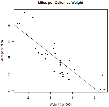
The lm function in R allows us to fit a range of linear models. However, we’ll start with a simple linear regression of one continuous dependent variable and one continuous independent variable. In this case, our model is of the form Y = α + β * X + ε, where the Y term represents our dependent variable, and X represents our independent variable(s). The α and β are parameters to be estimated and ε is our error term. For this hour, let’s use the mtcars data to fit simple models, starting with a linear regression of mpg versus wt, which can be visualized in Figure 16.1.
> plot(mtcars$wt, mtcars$mpg, main = "Miles per Gallon vs Weight",
+ xlab = "Weight (lb/1000)", ylab = "Miles per Gallon", pch = 16)

Note: Base Graphics
For this section, we will use the base graphics system to produce plots, because that is the system in which most model-fitting “diagnostic” plots are implemented.
This example creates a scatter plot of mpg versus wt. From the plot, it is clear that a relationship exists between mpg and wt that looks approximately linear, with miles per gallon reducing based on increased vehicle weights.
Fitting the Model
To create the plot in Figure 16.1, we stated our x and y variables explicitly using the $ syntax. However, we can also create the same basic plot using formula and data arguments, plot(mpg ~ wt, data = mtcars). The lm function works in much the same way. The first argument to lm (and, in fact, most model-fitting functions) is a “formula” defining the specific relationship to model. As with lattice graphics, we use the ~ symbol to establish a relationship as part of a formula. To specify a linear relationship between two variables, we use Y ~ X, which corresponds to a model of Y = α + β * X + ε. It should be noted, in particular, that specifying Y ~ X denotes a relationship that includes an intercept term (α). Let’s go ahead and fit our linear model of mpg versus wt using the lm function. We will save the output from the model fit as an object and print the value of the object.
> model1 <- lm(mpg ~ wt, data = mtcars) # Fit the model
> model1
Call:
lm(formula = mpg ~ wt, data = mtcars)
Coefficients:
(Intercept) wt
37.285 -5.344
Note: The data Argument
Note that lm, like the majority of model-fitting functions in R, accepts a data argument that specifies the data frame from which the model variables are taken. If preferred, we can omit this argument and fit the model by specifying vector inputs, such as lm(Y ~ X) or, in our example, lm(mtcars$mpg ~ mtcars$wt).
Tip: Removing the Intercept
As mentioned, the default behavior when specifying a model of Y ~ X is to include an intercept term. If appropriate, we can remove the intercept term by instead defining the formula as Y ~ X – 1.
Assessing a Model in R
In the previous section, we fitted a simple linear regression of mpg versus wt. Printing the resulting object from the lm function, we see a concise text output containing two elements:
![]() The “call” that was made to the function. (A model always knows how it was created.)
The “call” that was made to the function. (A model always knows how it was created.)
![]() The estimated coefficients of the model (
The estimated coefficients of the model (α = 37.285 and β = -5.344).
The next step is to assess whether our model is a “good” model and look for areas of improvement. To assess a model’s appropriateness, we can investigate the following:
![]() The overall measures of fit, such as the Residual Standard Error
The overall measures of fit, such as the Residual Standard Error
![]() Plots of “predicted” (or “fitted”) values and model “residuals” (where the residuals values are calculated by subtracting the fitted values from the observed responses)
Plots of “predicted” (or “fitted”) values and model “residuals” (where the residuals values are calculated by subtracting the fitted values from the observed responses)
![]() Metrics on the influence of each independent variable
Metrics on the influence of each independent variable
Clearly, the printed output from our model object provides very little insight into the model fit itself. For that, we need to use further functions that allow us to explore other aspects of our model.
Model Summaries
As seen in the previous section, the printed output from a model is rather concise, reporting only the function call and the estimated parameters. We can generate a more detailed textual output from our model using the summary function, which accepts a model object as the input. The output from this is shown in Listing 16.1.
LISTING 16.1 Output from Summary of Model
1: > summary(model1) # Summary of the lm model
2:
3: Call:
4: lm(formula = mpg ~ wt, data = mtcars)
5:
6: Residuals:
7: Min 1Q Median 3Q Max
8: -4.5432 -2.3647 -0.1252 1.4096 6.8727
9:
10: Coefficients:
11: Estimate Std. Error t value Pr(>|t|)
12: (Intercept) 37.2851 1.8776 19.858 < 2e-16 ***
13: wt -5.3445 0.5591 -9.559 1.29e-10 ***
14: ---
15: Signif. codes: 0 '***' 0.001 '**' 0.01 '*' 0.05 '.' 0.1 ' ' 1
16:
17: Residual standard error: 3.046 on 30 degrees of freedom
18: Multiple R-squared: 0.7528, Adjusted R-squared: 0.7446
19: F-statistic: 91.38 on 1 and 30 DF, p-value: 1.294e-10
As you can see, the summary function results in considerably more metrics. The information returned is shown in Table 16.1, which describes the output shown in Listing 16.1.

There are a small number of additional arguments we can provide to the summary function, including the correlation input, which allows us to additionally include the correlation matrix of estimated parameters, as shown in the following example. For more information, see the help file for ?summary.lm.
Model Diagnostic Plots
In Hour 13, “Graphics,” we introduced the plot function, which allows us to produce scatter plots of our data. In fact, we used the plot function earlier in this hour to create the scatter plot in Figure 16.1. We can also use the plot function to create diagnostic plots for model objects, such as our model1 object. By default, four diagnostic plots will be created, so we will first use the mfrow layout parameter to create a 2×2 plot surface that is displayed in Figure 16.2:
> par(mfrow = c(2, 2)) # Set up a 2x2 Graph Page
> plot(model1) # Create diagnostic plots for model1

The four plots created by the call to the plot function are described in Table 16.2.

Tip: Additional Arguments to plot
We can provide a number of additional arguments to plot. Most of these are concerned with the formatting of each plot (such as the id.n input, which controls the number of “extreme” values to be identified on each plot). Perhaps the most interesting is the which argument, which controls which plots are to be produced by plot. By default, which is set to c(1:3, 5), indicating the index of the four plots to be created. If, instead, we specify which = 1:6, the plot function will create six plots (the four described previously plus two that visualize Cook’s distance measures). For more information, see the help file for ?plot.lm.
Extracting Model Elements
R provides three functions that will return key elements of a linear model object (and, in fact, the majority of model types). The three functions are described in Table 16.3.

The use of these functions can be seen here:
> coef(model1) # Model coefficients
(Intercept) wt
37.285126 -5.344472
> head(resid(model1)) # Fitted Values
Mazda RX4 Mazda RX4 Wag Datsun 710
-2.2826106 -0.9197704 -2.0859521
Hornet 4 Drive Hornet Sportabout Valiant
1.2973499 -0.2001440 -0.6932545
> head(fitted(model1)) # Residuals (observed - fitted)
Mazda RX4 Mazda RX4 Wag Datsun 710
23.28261 21.91977 24.88595
Hornet 4 Drive Hornet Sportabout Valiant
20.10265 18.90014 18.79325
Let’s use the resid function to create scatter plots of our residuals versus the other nine variables from mtcars (seen in Figure 16.3):
> whichVars <- setdiff(names(mtcars), c("wt", "mpg")) # Names of other variables
in mtcars
> par(mfrow = c(3, 3)) # Set plot layout
> for (V in whichVars) { # Loop through create
scatter plots
+ plot(mtcars[[V]], resid(model1), main = V, xlab ="", pch = 16)
+ lines(loess.smooth(mtcars[[V]], resid(model1)), col = "red")
+ }

From these plots, it seems that there are other variables we should include in our model—we’ll do that later in this hour.
Models as List Objects
In the previous sections, you saw a number of ways of accessing information from a model:
![]() Printing the contents of the model object
Printing the contents of the model object
![]() Using the
Using the summary function to create a more detailed textual output
![]() Using the
Using the plot function to create a range of diagnostic plots
![]() Using functions
Using functions resid, coef, and fitted to extract key model elements
These approaches all use the information stored in the model object (returned from the call to lm). From the “Value” section of the lm help file (?lm), we can see that the function returns “an object of class lm,” which is a “list” containing a number of components. Because our object is, fundamentally, a list, we can show the names of its elements using the names function (as seen in Hour 4, “Multi-Mode Data Structures”). Let’s check the class of our model1 object and see the elements it contains:
> class(model1) # The class of model1
[1] "lm"
> is.list(model1) # Is model1 a list?
[1] TRUE
> names(model1) # The element names of model1
[1] "coefficients" "residuals" "effects" "rank"
[5] "fitted.values" "assign" "qr" "df.residual"
[9] "xlevels" "call" "terms" "model"
The “Value” section of the lm help file also describes these elements; this information can be seen in Table 16.4.

Given that our object is a list and we know the element names, we can directly extract elements using the $ symbol, as shown here:
> model1$coefficients # Model Coefficients
(Intercept) wt
37.285126 -5.344472
> quantile(model1$residuals, # Specific quantiles of residuals
+ probs = c(0.05, 0.5, 0.95))
5% 50% 95%
-3.8071897 -0.1251956 6.1794815
Model Summaries as List Objects
You have seen that the summary function allows us to produce a detailed textual summary of our model fit. In fact, the summary function (when applied to an lm object) also returns a list object that can be queried. This is shown in the following example:
> sModel1 <- summary(model1) # Summary of model1
> class(sModel1) # Class of summary object
[1] "summary.lm"
> is.list(sModel1) # Is it a list?
[1] TRUE
> names(sModel1) # Element names
[1] "call" "terms" "residuals" "coefficients"
[5] "aliased" "sigma" "df" "r.squared"
[9] "adj.r.squared" "fstatistic" "cov.unscaled"
> sModel1$adj.r.squared # Adjusted R Squared
[1] 0.7445939
> sModel1$sigma^2 # Estimate variance
[1] 9.277398
The elements of this object are described in Table 16.5 (taken from the summary.lm help file).

Adding Model Lines to Plots
At the start of this hour, we created a scatter plot of mpg vs. wt (refer to Figure 16.1). We can add a linear regression line to this plot based on our model fit using the abline function (which you also saw earlier in Hour 13). The following code adds a solid line representing our model fit; the resulting plot can be seen in Figure 16.4.
> plot(mtcars$wt, mtcars$mpg, main = "Miles per Gallon vs Weight",
+ xlab = "Weight (lb/1000)", ylab = "Miles per Gallon", pch = 16)
> abline(model1)
Caution: Additional Arguments to plot
When our models are more complex, involving multiple variables or nonlinear relations, a simple abline call will not work and other approaches must be taken. However, for simple models such as the one in this example, it works well.
Making Model Predictions
Once we have a model, we can make predictions using the predict function. If we supply only the model object to predict, then fitted values are returned:
> head(predict(model1)) # Model Predictions using model1
Mazda RX4 Mazda RX4 Wag Datsun 710
23.28261 21.91977 24.88595
Hornet 4 Drive Hornet Sportabout Valiant
20.10265 18.90014 18.79325
> head(fitted(model1)) # Fitted Values of model1
Mazda RX4 Mazda RX4 Wag Datsun 710
23.28261 21.91977 24.88595
Hornet 4 Drive Hornet Sportabout Valiant
20.10265 18.90014 18.79325
We can, instead, provide a data frame containing the set(s) of independent variables for which out-of-sample predictions are to be made. This data frame is supplied as the newdata input to predict, as shown here:
> wtDf <- data.frame(wt = 1:6) # Independent Variables
> predVals <- predict(model1, newdata = wtDf) # Make predictions using
model1
> data.frame(wt = wtDf$wt, Pred = round(predVals, 1)) # Form as data frame
wt Pred
1 1 31.9
2 2 26.6
3 3 21.3
4 4 15.9
5 5 10.6
6 6 5.2
Other arguments to the predict function allow us to customize our predictions in a number of ways. For example, we can use the se.fit and interval arguments to provide standard errors and confidence intervals related to our predictions, as shown here:
> predict(model1, newdata = wtDf, se.fit = TRUE, interval = "confidence")
$fit
fit lwr upr
1 31.940655 29.18042 34.700892
2 26.596183 24.82389 28.368481
3 21.251711 20.12444 22.378987
4 15.907240 14.49018 17.324295
5 10.562768 8.24913 12.876406
6 5.218297 1.85595 8.580644
$se.fit
1 2 3 4 5 6
1.3515519 0.8678067 0.5519713 0.6938618 1.1328743 1.6463754
$df
[1] 30
$residual.scale
[1] 3.045882
Multiple Linear Regression
Figure 16.3 showed a plot of the residuals from our model versus other variables in the mtcars data frame. We can include more than one independent variable in a model by separating variables by a + symbol on the right side of the formula. Therefore, we can specify a formula as Y ~ X1 + X2, which corresponds to a model of Y = α + β1 * X1 + β2 * X2 + ε. Here, α, β1 and β2 are parameters to be estimated and ε is our error term. Let’s define a new model including both wt and the hp variable:
> model2 <- lm(mpg ~ wt + hp, data = mtcars) # Fit new model
> summary(model2)
Call:
lm(formula = mpg ~ wt + hp, data = mtcars)
Residuals:
Min 1Q Median 3Q Max
-3.941 -1.600 -0.182 1.050 5.854
Coefficients:
Estimate Std. Error t value Pr(>|t|)
(Intercept) 37.22727 1.59879 23.285 < 2e-16 ***
wt -3.87783 0.63273 -6.129 1.12e-06 ***
hp -0.03177 0.00903 -3.519 0.00145 **
---
Signif. codes: 0 '***' 0.001 '**' 0.01 '*' 0.05 '.' 0.1 ' ' 1
Residual standard error: 2.593 on 29 degrees of freedom
Multiple R-squared: 0.8268, Adjusted R-squared: 0.8148
F-statistic: 69.21 on 2 and 29 DF, p-value: 9.109e-12
You can see from this output that the coefficient of the hp variable is significant at the 1% level, so including it would initially seem to be a good idea.
Updating Models
In the last example, we created a new model (model2) including two independent variables (wt and hp). It is common, when model fitting, to create a new model by varying the aspects of a previous model. That could include the following:
![]() Adding or removing a model term
Adding or removing a model term
![]() Removing outlying observations
Removing outlying observations
![]() Changing a model-fitting option
Changing a model-fitting option
Instead of creating new models directly, we can create new models by updating existing models with the update function. To achieve this, we supply an existing model and identify what to change. As an example, let’s re-create model2, this time using the update function:
> model2 <- update(model1, mpg ~ wt + hp) # Create model2 based on model1
> model2
Call:
lm(formula = mpg ~ wt + hp, data = mtcars)
Coefficients:
(Intercept) wt hp
37.22727 -3.87783 -0.03177
Although this example is very simple, when we have more complex models, this approach can be very efficient.
Tip: Updating Formula
When updating the model in this example, we specified the new formula as mpg ~ wt + hp. However, we can reduce the amount of typing using the period character to denote all formula elements of the previous model. Therefore, we could rewrite the previous example as follows:
> model2 <- update(model1, . ~ . + hp) # Create model2 based on model1
Again, when we have large models, this can be a far more efficient way of developing models.
Comparing Nested Models
In the previous section, we created a new model, model2, with an added term (hp). An initial look at the summary from model2 suggests that hp should be included in our model. Note that the independent variables in model1 are a subset of those in model2. The models are otherwise identical. In cases such as this, we say that model1 is nested within model2. Instead of looking at the models in isolation, we can compare two (or more) nested models using the following approaches:
![]() Creating comparative diagnostic plots
Creating comparative diagnostic plots
![]() Computing analysis of variance tables
Computing analysis of variance tables
Comparative Diagnostic Plots
Because we can access the information in each model, either directly or using functions such as resid and fitted, we can create plots that overlay data from two or more models. Let’s start by creating a plot of residuals vs. fitted values for each of our two models. The output can be seen in Figure 16.5.
> # Extract elements
> res1 <- resid(model1)
> fit1 <- fitted(model1)
> res2 <- resid(model2)
> fit2 <- fitted(model2)
> # Calculate axis range
> resRange <- c(-1, 1) * max(abs(res1), abs(res2))
> fitRange <- range(fit1, fit2)
> # Create plot for model1 > add points for model2
> plot(fit1, res1, xlim = fitRange, ylim = resRange,
+ col = "red", pch = 16, main = "Residuals vs Fitted Values",
+ xlab = "Fitted Values", ylab = "Residuals")
> points(fit2, res2, col = "blue", pch = 16)
> # Add reference and smooth lines
> abline(h = 0, lty = 2)
> lines(loess.smooth(fit1, res1), col = "red")
> lines(loess.smooth(fit2, res2), col = "blue")
> legend("bottomleft", c("mpg ~ wt", "mpg ~ wt + hp"), fill = c("red", "blue"))

We can use a similar approach to see how different models deal with variables in our data. For example, let’s see how the addition of the hp variable in model2 has helped to deal with the relationship between the model1 residuals and hp shown in Figure 16.3. The resulting plot can be seen in Figure 16.6.
> # Create plot for model1 > add points for model2
> plot(mtcars$hp, res1, ylim = resRange,
+ col = "red", pch = 16, main = "Residuals vs Fitted Values",
+ xlab = "Fitted Values", ylab = "Residuals")
> points(mtcars$hp, res2, col = "blue", pch = 16)
> # Add reference and smooth lines
> abline(h = 0, lty = 2)
> lines(loess.smooth(mtcars$hp, res1, span = .8), col = "red")
> lines(loess.smooth(mtcars$hp, res2, span = .8), col = "blue")
> legend("bottomleft", c("mpg ~ wt", "mpg ~ wt + hp"), fill = c("red", "blue"))

Analysis of Variance
We can create an analysis of variable table for one or more linear models using the anova functions. For this to make statistical sense, the models provided should be nested. For each model, the residual degrees of freedom and sum of squares is reported. In addition, an F test is performed for each step, with the p-value report. Let’s create an analysis of variance table to compare model1 and model2:
> anova(model1, model2)
Analysis of Variance Table
Model 1: mpg ~ wt
Model 2: mpg ~ wt + hp
Res.Df RSS Df Sum of Sq F Pr(>F)
1 30 278.32
2 29 195.05 1 83.274 12.381 0.001451 **
---
Signif. codes: 0 '***' 0.001 '**' 0.01 '*' 0.05 '.' 0.1 ' ' 1
You can see from the p-value (the value below Pr(>F)) that the inclusion of the hp variable significantly improved the model fit (assuming a p-value of 0.05).
Interaction Terms
We may wish to test whether there is a significant interaction term in the model. For example, we may hypothesize that wt has a different effect on mpg depending on differing values of hp. To test an interaction term, we specify it using the : symbol. Therefore, we can specify a formula as Y ~ X1 + X2 + X1:X2, which corresponds to a model of Y = α + β1 * X1 + β2 * X2 + β2 * X1 * X2 + ε. Here, α, β1, β2, and β3 are parameters to be estimated and ε is our error term. Let’s update model2 to include this interaction term.
> model3 <- update(model2, . ~ . + wt:hp)
> summary(model3)
Call:
lm(formula = mpg ~ wt + hp + wt:hp, data = mtcars)
Residuals:
Min 1Q Median 3Q Max
-3.0632 -1.6491 -0.7362 1.4211 4.5513
Coefficients:
Estimate Std. Error t value Pr(>|t|)
(Intercept) 49.80842 3.60516 13.816 5.01e-14 ***
wt -8.21662 1.26971 -6.471 5.20e-07 ***
hp -0.12010 0.02470 -4.863 4.04e-05 ***
wt:hp 0.02785 0.00742 3.753 0.000811 ***
---
Signif. codes: 0 '***' 0.001 '**' 0.01 '*' 0.05 '.' 0.1 ' ' 1
Residual standard error: 2.153 on 28 degrees of freedom
Multiple R-squared: 0.8848, Adjusted R-squared: 0.8724
F-statistic: 71.66 on 3 and 28 DF, p-value: 2.981e-13
Assess Addition of Interaction Term
From the preceding summary output, the interaction terms certainly seem highly significant, as are the other parameters when assessed in the presence of the interaction. Let’s compare our models with a quick graphic, seen in Figure 16.7. This time, we’ll add horizontal reference lines at the 5% and 95% residual quantiles.
> # Extract elements for model 3
> res3 <- resid(model3)
> fit3 <- fitted(model3)
> # Calculate axis range
> resRange <- c(-1, 1) * max(resRange, abs(res3))
> fitRange <- range(fitRange, fit3)
> # Create plot for model1 > add points for model2
> plot(fit1, res1, xlim = fitRange, ylim = resRange,
+ col = "red", pch = 16, main = "Residuals vs Fitted Values",
+ xlab = "Fitted Values", ylab = "Residuals")
> points(fit2, res2, col = "blue", pch = 16)
> points(fit3, res3, col = "black", pch = 16)
> # Add reference and smooth lines
> abline(h = 0, lty = 2)
> lines(loess.smooth(fit1, res1), col = "red")
> lines(loess.smooth(fit2, res2), col = "blue")
> lines(loess.smooth(fit3, res3), col = "black")
> # Add 5% and 95% reference lines for each model
> refFun <- function(res, col) abline(h = quantile(res, c(.05, .95)), col = col, lty = 3)
> refFun(res1, "red")
> refFun(res2, "blue")
> refFun(res3, "black")
> legend("bottomleft", c("mpg ~ wt", "mpg ~ wt + hp", "mpg ~ wt + hp + wt:hp"),
+ fill = c("red", "blue", "black"))

The addition of the interaction term certainly seems to have improved our model. As a last check, let’s create an analysis of the variance table for our three models:
> anova(model1, model2, model3)
Analysis of Variance Table
Model 1: mpg ~ wt
Model 2: mpg ~ wt + hp
Model 3: mpg ~ wt + hp + wt:hp
Res.Df RSS Df Sum of Sq F Pr(>F)
1 30 278.32
2 29 195.05 1 83.274 17.969 0.0002207 ***
3 28 129.76 1 65.286 14.088 0.0008108 ***
---
Signif. codes: 0 '***' 0.001 '**' 0.01 '*' 0.05 '.' 0.1 ' ' 1
In this case, the F test and corresponding p-values are derived by testing each model against the largest model provided (in this case model3). The significance of the two comparisons supports our claim that model3 is an improvement over each of the previous models.
Tip: Linear Combinations Including Interactions
In the previous section, you saw that we can create models with linear combinations of variables and interaction terms using a formula such as Y ~ X1 + X2 + X1:X2. Another way of writing this is as Y ~ X1*X2, which expands to Y ~ X1 + X2 + X1:X2. This works for any number of variables; for example, we could use Y ~ X1*X2*X3 to create a model of Y ~ X1 + X2 + X3 + X1:X2 + X1:X3 + X2:X3 + X1:X2:X3!
Factor Independent Variables
So far in this hour, we have used only continuous independent variables. In fact, the lm function allows us to include factor variables as independent variables. In the mtcars dataset, there are a number of variables we could treat as factor variables, each of which may be influential in our model. Let’s first look at the residuals from our current model (model3) versus some of these factor variables, seen in Figure 16.8. Let’s focus on three variables that we’ll treat as categorical:
![]() The
The vs variable, an indicator for whether the engine is a “straight” (0) or “V” engine (1)
![]() The
The am variable, an indicator of the transmission type: 0 for automatic, 1 for manual.
![]() The
The cyl variable, which contains the number of cylinders (4, 6, or 8).

These variables are actually stored as numeric, so we will need to convert them to factors first:
> par(mfrow = c(1, 3))
> plot(factor(mtcars$vs), resid(model3), col = "red",
+ xlab = "0 = Straight Engine 1 = 'V Engine'", ylab = "Residuals",
+ main = "Residuals versus
'V Engine' Flag")
> plot(factor(mtcars$am), resid(model3), col = "red",
+ xlab = "0 = Automatic 1 = Manual", ylab = "Residuals",
+ main = "Residuals versus
Transmission Type")
> plot(factor(mtcars$cyl), resid(model3), col = "red",
+ xlab = "Number of Cylinders", ylab = "Residuals",
+ main = "Residuals versus
Number of Cylinders")
Including Factors
Let’s add cyl to our model and see what impact it has. To achieve this, we will specify cyl as a factor variable; otherwise, it would be handled as a continuous independent variable.
> model4 <- update(model3, . ~ . + factor(cyl))
> summary(model4)
Call:
lm(formula = mpg ~ wt + hp + factor(cyl) + wt:hp, data = mtcars)
Residuals:
Min 1Q Median 3Q Max
-3.5309 -1.6451 -0.4154 1.3838 4.4788
Coefficients:
Estimate Std. Error t value Pr(>|t|)
(Intercept) 47.337329 4.679790 10.115 1.67e-10 ***
wt -7.306337 1.675258 -4.361 0.000181 ***
hp -0.103331 0.031907 -3.238 0.003274 **
factor(cyl)6 -1.259073 1.489594 -0.845 0.405685
factor(cyl)8 -1.454339 2.063696 -0.705 0.487246
wt:hp 0.023951 0.008966 2.671 0.012865 *
---
Signif. codes: 0 '***' 0.001 '**' 0.01 '*' 0.05 '.' 0.1 ' ' 1
Residual standard error: 2.203 on 26 degrees of freedom
Multiple R-squared: 0.888, Adjusted R-squared: 0.8664
F-statistic: 41.21 on 5 and 26 DF, p-value: 1.503e-11
The coefficients are reported for cyl = 6 and cyl = 8, with the first level (cyl = 4) taken as the baseline. This is because “treatment” contrasts are the default contrast method for unordered factors. The treatment “contrast” method contrasts each level with a baseline level, taken (by default) as the first level of the variable.
Tip: Control of Contrasts
There are five contrast methods available in R: contr.treatment (the default), contr.sum, contr.poly, contr.helmert, and contr.SAS. Each of the contrast options is represented by a function that is used to create a contrast matrix of the appropriate size. The following is an example for a factor with three levels:
> contr.treatment(3) # Matrix of dummy variables to use for a 3-level factor
(like cyl)
2 3
1 0 0
2 1 0
3 0 1
We view and set the default contrast using options("contrasts").
From the model output, it is clear that the cyl variable is not significant in the model. This is further supported by an analysis of variance, which shows that very little additional variance is explained with the addition of the cyl variable between model3 and model4:
> anova(model1, model2, model3, model4)
Analysis of Variance Table
Model 1: mpg ~ wt
Model 2: mpg ~ wt + hp
Model 3: mpg ~ wt + hp + wt:hp
Model 4: mpg ~ wt + hp + factor(cyl) + wt:hp
Res.Df RSS Df Sum of Sq F Pr(>F)
1 30 278.32
2 29 195.05 1 83.274 17.1624 0.0003219 ***
3 28 129.76 1 65.286 13.4552 0.0011040 **
4 26 126.16 2 3.606 0.3716 0.6932114
---
Signif. codes: 0 '***' 0.001 '**' 0.01 '*' 0.05 '.' 0.1 ' ' 1
One interesting thing from the summary output, however, is that the significance of the hp variable (and the interaction term) were slightly lessened with the inclusion of cyl. The reason for this is that hp and cyl are highly correlated (as seen in Figure 16.9), so the “information” provided by hp is very similar to that supplied by cyl.
> plot(factor(mtcars$cyl), mtcars$hp, col = "red",
+ xlab = "Number of Cylinders", ylab = "Gross Horsepower",
+ main = "Gross Horsepower vs Number of Cylinders")

We could, as a next step, replace hp with cyl in the model and also look at interaction terms between wt and cyl.
Variable Transformations
If we look back at Figure 16.1, which plotted mpg versus wt, there is a suggestion of curvature. Let’s see this plot again, this time alongside of plot of log(mpg) versus wt. This can be seen in Figure 16.10.
> par(mfrow = c(1, 2))
> plot(mtcars$wt, mtcars$mpg, pch = 16, xlab = "Weight (lb/1000)",
+ ylab = "Miles per Gallon", main = "MPG Gallon versus Weight")
> lines(loess.smooth(mtcars$wt, mtcars$mpg), col = "red")
> plot(mtcars$wt, log(mtcars$mpg), pch = 16, xlab = "Weight (lb/1000)",
+ ylab = "log(Miles per Gallon)", main = "Logged MPG versus Weight")
> lines(loess.smooth(mtcars$wt, log(mtcars$mpg)), col = "red")

Based on this visualization, we may decide to try to model logged miles per gallon. If we want to transform any of our dependent or independent variables, we can apply a transformation function directly in the formula. Let’s create a simple model of logged miles per gallon versus weight horsepower. We’ll look at the detailed summary output and also create some diagnostic plots (seen in Figure 16.11).
> lmodel1 <- lm(log(mpg) ~ wt, data = mtcars)
> summary(lmodel1)
Call:
lm(formula = log(mpg) ~ wt, data = mtcars)
Residuals:
Min 1Q Median 3Q Max
-0.210346 -0.085932 -0.006136 0.061335 0.308623
Coefficients:
Estimate Std. Error t value Pr(>|t|)
(Intercept) 3.83191 0.08396 45.64 < 2e-16 ***
wt -0.27178 0.02500 -10.87 6.31e-12 ***
---
Signif. codes: 0 '***' 0.001 '**' 0.01 '*' 0.05 '.' 0.1 ' ' 1
Residual standard error: 0.1362 on 30 degrees of freedom
Multiple R-squared: 0.7976, Adjusted R-squared: 0.7908
F-statistic: 118.2 on 1 and 30 DF, p-value: 6.31e-12
> par(mfrow = c(2, 2)) # Set plot layout
> plot(lmodel1) # Create diagnostics plots

If we want to overlay this model onto our original data, it is better to exponentiate some predicted results and use the lines function to add the line to the plot. Let’s compare the original model of mpg vs. wt with the new model of log(mpg) vs. wt. The output can be seen in Figure 16.12.
> plot(mtcars$wt, mtcars$mpg, pch = 16, xlab = "Weight (lb/1000)",
+ ylab = "Miles per Gallon", main = "MPG Gallon versus Weight")
> abline(model1, col = "red") # Add (straight) model line (based on earlier
model1 object)
> wtVals <- seq(min(mtcars$wt), max(mtcars$wt), length = 50) # Weights to
predict at
> predVals <- predict(lmodel1, newdata = data.frame(wt = wtVals)) # Make
predictions
> lines( wtVals, exp(predVals), col = "blue") # Add (log) model
line
> legend("topright", c("mpg ~ wt", "log(mpg) ~ wt"), fill = c("red", "blue"))

Caution: Inhibiting Interpretation
If we want to transform dependent or independent variables, it is worth noting that some model formula syntax has special meaning. For example, if we wanted to model a response Y against a continuous variable X, we’d use Y ~ X. However, if we instead wanted to model Y against “X – 1” (the values of X with 1 subtracted), we might try Y ~ X – 1. However, this syntax denotes a model of Y against X without an intercept term. If we literally want to model Y against “X – 1”, we need to include the I function, which inhibits the interpretation of the formula. Therefore, our formula would become Y ~ I(X – 1). For more information on the formula syntax, including the I function, see the ?formula help file.
R and Object Orientation
In the preceding sections, we used functions such as summary and plot to understand our models. However, we have seen these functions used in earlier hours to summarize and graph other objects. In addition to the outputs from summary related to the preceding models, consider the following uses of the summary function:
> summary(mtcars$mpg) # Summary of a numeric vector
Min. 1st Qu. Median Mean 3rd Qu. Max.
10.40 15.42 19.20 20.09 22.80 33.90
> summary(factor(mtcars$cyl)) # Summary of a factor vector
4 6 8
11 7 14
> summary(mtcars[,1:4]) # Summary of a data frame
mpg cyl disp hp
Min. :10.40 Min. :4.000 Min. : 71.1 Min. : 52.0
1st Qu.:15.43 1st Qu.:4.000 1st Qu.:120.8 1st Qu.: 96.5
Median :19.20 Median :6.000 Median :196.3 Median :123.0
Mean :20.09 Mean :6.188 Mean :230.7 Mean :146.7
3rd Qu.:22.80 3rd Qu.:8.000 3rd Qu.:326.0 3rd Qu.:180.0
Max. :33.90 Max. :8.000 Max. :472.0 Max. :335.0
In these examples, the summary function produces different output depending on the type of object it is provided. The summary help file describes it as a “generic” function, which provides “methods” for many “classes” of objects. But what does this mean?
Object Orientation
Many features of the R language are based on the object-oriented programming paradigm. To describe object orientation, let’s consider the following:
![]() If someone asks us to open a door, we would turn the handle.
If someone asks us to open a door, we would turn the handle.
![]() If someone asks us to open a bottle, we would twist the top.
If someone asks us to open a bottle, we would twist the top.
![]() If someone asks us to open a box, we would lift the lid.
If someone asks us to open a box, we would lift the lid.
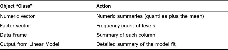
For each of these statements, the “command” is the same: “open.” However, we behave differently based on the type of object we are to “open.” The idea behind object-oriented programming is similar. Here, the “command” is called a “method,” and the “type” of object is called the “class” of the object. We have seen a number of examples of this behavior in this hour, such as the previous summary function uses, which are described in Table 16.6.
R contains a number of systems for object-oriented programming. The majority of the statistical modeling functionality available in R is based on the “S3” system, which implements generic functions and uses a simple naming convention. When a method is called, the class of the object is appended to the name of the method, separated by a period character, and the process is redirected to this function. So when we perform a summary of an object of class “factor,” we instead call function summary.factor, as shown in the following example:
> cylFactor <- factor(mtcars$cyl)
> class(cylFactor)
[1] "factor"
> summary(cylFactor)
4 6 8
11 7 14
> summary.factor(cylFactor)
4 6 8
11 7 14
Note: Using R Classes
In Hour 21, “Writing R Classes,” and Hour 22, “Formal Class Systems,” we will look more closely at S3 and other object-oriented programming systems provided by R.
Linear Model Methods
For most of this hour, we’ve been using functions such as summary and plot to evaluate linear models, which we fitted with the lm function. The “class” of these objects can be seen with the class function:
> class(model1)
[1] "lm"
> class(model2)
[1] "lm"
> class(model3)
[1] "lm"
> class(model4)
[1] "lm"
Using this fact, we now know the names of the functions we have been calling throughout the previous sections of this hour, many of which are summarized in Table 16.7.

Perhaps the most important reason to understand this mechanism is to know which is the relevant help file to read to understand the options available to us. For example, if we’re using the summary function for an lm object, we know that summary.lm is the help file we need to refer to.
Summary
In this hour, you saw how to fit a series of simple linear models in R. This includes the way in which we define our linear model via the use of a “formula” as well as a number of ways to assess the appropriateness of our model using textual and graphical means. We also introduced the concept of object-oriented programming by looking at the behavior of generic functions such as print, summary, and plot when given linear model outputs. Although we focused on linear models in this hour, the concepts and approach we used is similar across a wide range of statistical models provided by R. In the next hour, we’ll look at some of these models and see how similar the approach is to the fitting of linear models covered in this hour.
A. Yes. Other types of residuals (such as Pearson and partial residuals) can be also be returned from the resid function. See the ?residuals.lm help file for more information.
Q. What other high-level metrics relating to model fit are available?
A. A number of additional metrics are available, such as Akaike’s Information Criteria (?AIC), Bayesian Information Criteria (?BIC), and Log-Likelihood (?logLik). This is not an exhaustive list, and we recommend searching the www.r-project.org site for specific methods if they have not been covered here.
Q. How do I extract the variance-covariance matrix of model parameters?
A. The vcov function allows you to extract the variance-covariance matrix of parameters given a model.
Q. How does lm deal with missing values?
A. The handling of missing values in lm is controlled by the na.action argument. By default, the na.action argument is set to na.omit, which removes rows including at least one missing based on the variables involved in the model.
Q. Can I perform polynomial regression using lm?
A. Yes. You can include independent variables in a polynomial manner. However, care must be taken because the ^ symbol in a formula has a particular meaning (it represents parameter crossing, as described in the ?formula help page). Therefore, to include variables in a polynomial manner you need the I function (for example, mpg ~ wt + I(wt^2)). An alternative approach is to use the poly function, which allows you to specify this as mpg ~ poly(wt, 2, raw = T).
Q. Is there functionality for stepwise regression in R?
A. Yes. The step function can be used to perform stepwise regression, which uses AIC as the basis for deciding which steps to take.
Workshop
The workshop contains quiz questions and exercises to help you solidify your understanding of the material covered. Try to answer all questions before looking at the “Answers” section that follows.
Quiz
1. How can we fit a model of Y against X without an intercept term?
2. What would a formula of Y ~ X1*X2 denote?
3. Which function can you use to extract the residuals from a model fit?
4. What help file would you refer to if you wanted to control the behavior of the plot function when producing diagnostic plots of a linear model?
5. What are the default contrast methods in R?
Answers
1. You would use Y ~ X – 1.
2. This denotes a model of Y against X1, X2 and the interaction of X1 and X2. Therefore, Y ~ X1*X2 is equivalent to Y ~ X1 + X2 + X1:X2.
3. You can use the resid function to extract residuals from a linear model.
4. If you are using the plot function with an object of class “lm” (which contains a linear model output), then the plot.lm help file would be the one to refer to.
5. The default contrast methods for an (unordered) factor variable in R are “treatment” contrasts, where the first level of the factor is taken as the baseline (as described in the ?contr.treatment help file).
Activities
1. Using the airquality data frame, fit a linear model of Ozone versus Wind.
2. Create detailed textual summaries and diagnostic plots to assess your model fit.
3. Use the update function to add Temp as an independent variable. Evaluate your new model and create an analysis of variance of these nested models.
4. Assess the inclusion of an interaction term (Wind:Temp) in your model.
5. Add Month as a categorical independent variable in your model.