
Chapter 2
MIMO System and Channel Models
2.1 MIMO System Model
In wireless communications, a transmitter is communicating with a receiver through free‐space medium. The transmitter is generally called the input as it transmits data into the communication link. The receiver is called the output as it receives transmitted data from the input. Depending on the number of antennas at both transmitter and receiver, several link configurations can be found. The simplest configuration is single‐input single‐output (SISO), where both transmitter and receiver each equipped with single antenna. If the transmitter has more than one antenna and communicates with single antenna receiver, a multiple‐input single‐output (MISO) configuration is conceived. If the receiver has more than one antenna and receives signal from a single antenna transmitter, a single‐input multiple‐output (SIMO) configuration is formed. Finally, if both transmitter and receiver have multiple antennas, a multiple‐input multiple‐output (MIMO) configuration is established.
In Figure 2.1, MIMO system model with ![]() transmit antennas and
transmit antennas and ![]() receive antennas is depicted.
receive antennas is depicted.

Figure 2.1 General MIMO system model with  transmit antennas and
  receive antennas.
This system can be represented by the following discrete time model:

which can be simplified to
where ![]() is the
is the ![]() ‐length transmitted vector,
‐length transmitted vector, ![]() is an
is an ![]() ‐length additive white Gaussian noise (AWGN) seen at the receiver input,
‐length additive white Gaussian noise (AWGN) seen at the receiver input, ![]() is an
is an ![]() MIMO channel matrix representing the path gains
MIMO channel matrix representing the path gains ![]() between transmit antenna
between transmit antenna ![]() and receive antenna
and receive antenna ![]() , and
, and ![]() is the
is the ![]() ‐length vector received signal.
‐length vector received signal.
The transmitted vector ![]() is created from the source data bit using a MIMO encoder, where arbitrary modulation techniques such as quadrature amplitude modulation (QAM), phase shift keying (PSK), or others are used by the MIMO encoder. The noise is generally modeled as a complex Gaussian noise that is temporally and spatially white with zero mean and a covariance matrix of
is created from the source data bit using a MIMO encoder, where arbitrary modulation techniques such as quadrature amplitude modulation (QAM), phase shift keying (PSK), or others are used by the MIMO encoder. The noise is generally modeled as a complex Gaussian noise that is temporally and spatially white with zero mean and a covariance matrix of ![]() , where
, where ![]() , with
, with ![]() denoting the noise power spectral density and
denoting the noise power spectral density and ![]() is the channel bandwidth. Also and when comparing systems with different configurations, the total transmit power from any number of transmit antennas is the same and for simplicity assumed to be 1. Therefore, the average signal‐to‐noise‐ratio (SNR) at each receive antenna (
is the channel bandwidth. Also and when comparing systems with different configurations, the total transmit power from any number of transmit antennas is the same and for simplicity assumed to be 1. Therefore, the average signal‐to‐noise‐ratio (SNR) at each receive antenna (![]() ), under unity channel gain assumptions, is given by SNR
), under unity channel gain assumptions, is given by SNR ![]() . At the receiver, the optimum maximum‐likelihood (ML) detector can be used to decode the transmitted messages as [111],
. At the receiver, the optimum maximum‐likelihood (ML) detector can be used to decode the transmitted messages as [111],
where ![]() denotes the estimated transmitted symbol,
denotes the estimated transmitted symbol, ![]() is the estimated channel matrix at the receiver,
is the estimated channel matrix at the receiver, ![]() is the frobenius norm, and
is the frobenius norm, and ![]() is a possible transmitted vector from
is a possible transmitted vector from ![]() , where
, where ![]() is a set containing all possible transmitted vectors combinations between transmit antennas and data symbols.1
is a set containing all possible transmitted vectors combinations between transmit antennas and data symbols.1
The ML decoder in (2.3) searches the transmitted vectors space and selects the vector that is closest to the received signal vector ![]() as the most probable transmitted vector. The closer the two vectors from the set
as the most probable transmitted vector. The closer the two vectors from the set ![]() to each others, the higher the probability of error. Therefore, a better design is to place the vectors as far apart from each other as possible. This can be done also through proper design of the MIMO channel matrix
to each others, the higher the probability of error. Therefore, a better design is to place the vectors as far apart from each other as possible. This can be done also through proper design of the MIMO channel matrix ![]() . Also, the computational complexity of encoding and decoding should be practical, systems with higher complexity tends to perform better.
. Also, the computational complexity of encoding and decoding should be practical, systems with higher complexity tends to perform better.
2.2 Spatial Multiplexing MIMO Systems
The first proposed spatial multiplexing (SMX) MIMO system was vertical Bell Labs layered space time (V‐BLAST) system [112]. Later on, horizontal Bell Labs layered space time (H‐BLAST) system was proposed [113]. In these systems, the input data stream is de‐multiplexed into ![]() parallel substreams. Each substream contains an independent data that will be transmitted from a single transmit antenna. In general wireless systems, channel coding and interleaving are generally applied. Based on the applied coding scheme, the different Bell Labs layered space time (BLAST) configurations are named. The H‐BLAST took its name because the channel coding is applied horizontally on each substream. The earlier V‐BLAST scheme called vertical since uncoded data symbol was viewed as one vector symbol. The transmitted streams from multiple transmit antennas are cochannel signals that share the same time and frequency slots. As such, the schemes mainly aim at decorrelating the received signals to retrieve the transmitted data. Each receive antenna observes a superposition of the transmitted signals, and the major task at the receiver is to resolve the inter‐channel interference (ICI) between the transmitted symbols. The optimum solution is to use ML receiver as in (2.3). The ML compares the received signals with all possible transmitted signal vectors that are modified by the channel matrix and selects the optimal codeword. The problem of ML algorithm is the high complexity required to search over all possible combinations. Therefore, initial systems targeted other low complexity receiver such as sphere decoder (SD) algorithm [114] and the multiple variants of it proposed in [115]. The V‐BLAST receiver was another low‐complexity receiver that applies a successive interference cancellation technique with optimum ordering (OR‐SIC). The optimal detection order is from the strongest symbol to the weakest one. The idea is to detect the strongest symbol first. Then, canceling the effect of this symbol from all received signals and detects the next strongest symbol and so on. The process is repeated until all symbols are detected. Details of this scheme can be found in [71, 112].
parallel substreams. Each substream contains an independent data that will be transmitted from a single transmit antenna. In general wireless systems, channel coding and interleaving are generally applied. Based on the applied coding scheme, the different Bell Labs layered space time (BLAST) configurations are named. The H‐BLAST took its name because the channel coding is applied horizontally on each substream. The earlier V‐BLAST scheme called vertical since uncoded data symbol was viewed as one vector symbol. The transmitted streams from multiple transmit antennas are cochannel signals that share the same time and frequency slots. As such, the schemes mainly aim at decorrelating the received signals to retrieve the transmitted data. Each receive antenna observes a superposition of the transmitted signals, and the major task at the receiver is to resolve the inter‐channel interference (ICI) between the transmitted symbols. The optimum solution is to use ML receiver as in (2.3). The ML compares the received signals with all possible transmitted signal vectors that are modified by the channel matrix and selects the optimal codeword. The problem of ML algorithm is the high complexity required to search over all possible combinations. Therefore, initial systems targeted other low complexity receiver such as sphere decoder (SD) algorithm [114] and the multiple variants of it proposed in [115]. The V‐BLAST receiver was another low‐complexity receiver that applies a successive interference cancellation technique with optimum ordering (OR‐SIC). The optimal detection order is from the strongest symbol to the weakest one. The idea is to detect the strongest symbol first. Then, canceling the effect of this symbol from all received signals and detects the next strongest symbol and so on. The process is repeated until all symbols are detected. Details of this scheme can be found in [71, 112].
In this book, SMX MIMO systems will be used as a benchmark system for comparison purposes with SMTs. The ML optimum decoder from (2.3) will be considered.
2.3 MIMO Capacity
Before 1948, it was widely believed that the only way to reduce the probability of error of a wireless communication system was to reduce the transmission data rate for fixed power and bandwidth. In 1948, Shannon showed that this belief is incorrect, and lower probability of error can be achieved through intelligent coding of the information. However, there is a maximum limit of data rate, called the capacity of the channel, for which this can be done. If the transmission rate exceeds the channel capacity, it will be impossible to derive the probability of error to zero [3].
The channel capacity is, therefore, a measure of the maximum amount of information that can be transmitted over the channel and received with no errors at the receiver [25],
where ![]() is the mutual information between the transmitted vector space
is the mutual information between the transmitted vector space ![]() and the received vector space
and the received vector space ![]() and the maximization is carried over the choice of the probability distribution function (PDF) of
and the maximization is carried over the choice of the probability distribution function (PDF) of ![]() .
.
In an AWGN channel and for SISO transmission of complex symbols, the channel capacity is given by [116],
The ergodic capacity of a SISO system over a slow fading random channel, assuming full channel state information (CSI) at the receiver side only, is given by [25, 116],
where ![]() is the squared magnitude of the channel coefficient, and
is the squared magnitude of the channel coefficient, and ![]() is the expectation operator. As the number of receiver antenna increases, the statistics of capacity improves. The capacity,
is the expectation operator. As the number of receiver antenna increases, the statistics of capacity improves. The capacity, ![]() in (2.6), is often referred to as the error‐free spectral efficiency, or the data rate that can be sustained reliably over the link [4].
in (2.6), is often referred to as the error‐free spectral efficiency, or the data rate that can be sustained reliably over the link [4].
In a SIMO system with an ![]() receiver antennas, there exist
receiver antennas, there exist ![]() various copies of the faded signal at the receiver. If these signals are, on average, the same amplitude, then they may be added coherently to produce an
various copies of the faded signal at the receiver. If these signals are, on average, the same amplitude, then they may be added coherently to produce an ![]() increase in signal power. Of course, there are
increase in signal power. Of course, there are ![]() sets of noise that will add together as well. Fortunately, noise adds incoherently to create only an
sets of noise that will add together as well. Fortunately, noise adds incoherently to create only an ![]() ‐fold increase in the noise power. Thus, there is still a net overall increase in SNR by
‐fold increase in the noise power. Thus, there is still a net overall increase in SNR by ![]() compared to SISO systems. Following this, the ergodic channel capacity of this system is [117],
compared to SISO systems. Following this, the ergodic channel capacity of this system is [117],
where in SIMO system, the channel matrix ![]() can be reduced to an
can be reduced to an ![]() ‐length channel vector
‐length channel vector ![]() , and
, and ![]() is the Hermitian operator.
is the Hermitian operator.
In a MISO system, where the transmitter is equipped with multiple antennas, whereas the receiver has single antenna, a special design of the transmit signal needs to exist for any possible advantages. Without precoding of transmitted data, received data from the multiple antennas will interfere at the receiver input and the capacity will be zero. Special techniques such as space–time coding (STC), repetition coding, and others are used in such topologies. The aim is to create orthogonal transmitted data that can be decoded by the receiver under a total power constraint; i.e. the transmit power is divided among existing transmit antennas. With such precoding, orthogonal signals are transmitted and the channel capacity is [4],

where in the case of MISO channels, ![]() is
is ![]() ‐length channel vector.
‐length channel vector.
Having ![]() antennas at the transmitter and
antennas at the transmitter and ![]() antennas at the receiver results in a MIMO configuration as discussed earlier. The ergodic capacity for a MIMO system over uncorrelated channel paths assuming equal total power transmission as in SISO systems is given by [25, 71, 116, 117],2
antennas at the receiver results in a MIMO configuration as discussed earlier. The ergodic capacity for a MIMO system over uncorrelated channel paths assuming equal total power transmission as in SISO systems is given by [25, 71, 116, 117],2

In order to interpret (2.9), let ![]() be the singular value decomposition (SVD) of the channel matrix
be the singular value decomposition (SVD) of the channel matrix ![]() .
. ![]() and
and ![]() are unitary matrices.
are unitary matrices. ![]() is a diagonal matrix of
is a diagonal matrix of ![]() of
of ![]() with
with ![]() and
and ![]() being the positive eigenvalues of
being the positive eigenvalues of ![]() . Rewriting (2.9) as
. Rewriting (2.9) as


Figure 2.2 Ergodic MIMO capacity for different antenna configurations. Capacity improves with larger antenna configurations.
The result of ![]() is a diagonal matrix containing the positive eigenvalues of
is a diagonal matrix containing the positive eigenvalues of ![]() . The diagonal elements are given by
. The diagonal elements are given by ![]() , where
, where ![]() is the rank of the channel matrix. Substituting this in (2.10) and using the identity
is the rank of the channel matrix. Substituting this in (2.10) and using the identity ![]() for matrices
for matrices ![]() and
and ![]() [111], and
[111], and ![]() simplifies (2.10) to
simplifies (2.10) to

It is shown in Figure 2.2 that using multiple antennas increases the ergodic capacity. The capacity increases with the increasing number of transmit antennas, receive antennas, or by increasing both of them at the same time.
2.4 MIMO Channel Models
Propagating signals from transmitter to receiver arrives from multipaths and suffer from multipath fading. The combined signals at the receiver are random in nature, and the received signal power changes over a period of time. The propagation channel consists of static or moving reflecting objects, and scatterers that create a randomly changing environment. If the channel has a constant gain and linear phase response over a bandwidth that is greater than the bandwidth of the transmitted signal, it is called flat fading or frequency nonselective fading channel [118]. This specific bandwidth is generally called the Coherence bandwidth and is a statistical measure of the range of frequencies over which the channel can be considered flat.
The movement of the transmitter, receiver, or the surrounding environment results in a random frequency modulation due to different Doppler shifts on each of the multipath components. Hence, a spectral broadening at the receiver side occurs and is measured by the Doppler spread, which is defined as the range of frequencies over which the received Doppler spectrum is not zero [119, 120].
Based on time and frequency statistics, fading channels can be classified into flat and frequency selective according to their time changes and slow and fast according to their frequency variations. These two phenomena are independent and result in the following fading types [121]:
- Flat slow fading or frequency nonselective slow fading: when the bandwidth of the signal is smaller than the coherence bandwidth of the channel and the signal duration is smaller than the coherence time of the channel. The coherence time is the duration of time in which the channel impulse response is effectively invariant.
- Flat fast fading or frequency nonselective fast fading: when the bandwidth of the signal is smaller than the coherence bandwidth of the channel and the signal duration is larger than the coherence time of the channel.
- Frequency selective slow fading: when the bandwidth of the signal is larger than the coherence bandwidth of the channel and the signal duration is smaller than the coherence time of the channel.
- Frequency selective fast fading: when the bandwidth of the signal is larger than the coherence bandwidth of the channel and the signal duration is larger than the coherence time of the channel.
The propagation environment plays a dominant role in determining the capacity of the MIMO channel. In what follows, several MIMO channel models are discussed.
2.4.1 Rayleigh Fading
The Rayleigh fading distribution is generally considered when the transmitter and receiver have no line‐of‐sight (LOS) [122, 123]. As such, the sum of all scattered and reflected components of the complex received signal is modeled as a zero mean complex Gaussian random process given by ![]() . Hence, the phase of the random process
. Hence, the phase of the random process ![]() takes an uniform distribution, and is given by
takes an uniform distribution, and is given by
where ![]() if
if ![]() and zero otherwise. Furthermore, the amplitude takes a Rayleigh distribution given by
and zero otherwise. Furthermore, the amplitude takes a Rayleigh distribution given by

where ![]() denotes the set of all positive real numbers.
denotes the set of all positive real numbers.
2.4.2 Nakagami‐ (Rician Fading)
If the transmitter and receiver can see each other through a LOS path, the channel amplitude gain is characterized by a Rician distribution, and the channel is said to exhibit Rician fading [120, 123, 124]. The Rician fading MIMO channel matrix can be modeled as the sum of a LOS matrix and a Rayleigh fading channel matrix as [123],

where ![]() is the Rician
is the Rician ![]() ‐factor. The Rician
‐factor. The Rician ![]() ‐factor is defined as the ratio of the LOS and the scatter power components. There are two contrasting prototypes of
‐factor is defined as the ratio of the LOS and the scatter power components. There are two contrasting prototypes of ![]() for a MIMO channel and unipolarized antennas. The first one is a matrix with all elements being one, which can be applied when the distance between the transmit antennas and the receive antennas is much larger than the spacing between the transmit antennas and the receive antennas. The second alternative is for the case when the distance between the transmit antennas and the receive antennas is comparable to the spacing between the transmit antennas and/or the receive antennas. The LOS component of the channel matrix, assuming
for a MIMO channel and unipolarized antennas. The first one is a matrix with all elements being one, which can be applied when the distance between the transmit antennas and the receive antennas is much larger than the spacing between the transmit antennas and the receive antennas. The second alternative is for the case when the distance between the transmit antennas and the receive antennas is comparable to the spacing between the transmit antennas and/or the receive antennas. The LOS component of the channel matrix, assuming ![]() for instance, is then given by
for instance, is then given by

Perfect orthogonality of this channel matrix requires specific antenna locations and geometry. Therefore, ![]() is likely only in multibase operations when transmit (or receive) antennas are located at different base stations [111].
is likely only in multibase operations when transmit (or receive) antennas are located at different base stations [111].
In Rician fading channel, the capacity of the MIMO system depends on the value of the Rician ![]() ‐factor and on the channel geometry. When the value of
‐factor and on the channel geometry. When the value of ![]() is low, the random matrix
is low, the random matrix ![]() has more influence than
has more influence than ![]() , resulting in an expression of the MIMO capacity similar to (2.11). However, when the value of
, resulting in an expression of the MIMO capacity similar to (2.11). However, when the value of ![]() is high, the LOS component of the channel matrix dominates and the capacity depends on the channel geometry of the LOS component. As discussed before, there exist two contrasting prototypes of
is high, the LOS component of the channel matrix dominates and the capacity depends on the channel geometry of the LOS component. As discussed before, there exist two contrasting prototypes of ![]() for a MIMO channel. The second one,
for a MIMO channel. The second one, ![]() , clearly outperforms the first channel with an increasing
, clearly outperforms the first channel with an increasing ![]() ‐factor. This is because the second matrix is orthogonal while the first one is rank‐deficient. Hence, the geometry of the LOS component of the channel matrix plays a critical rule in channel capacity at high Rician factor [125].
‐factor. This is because the second matrix is orthogonal while the first one is rank‐deficient. Hence, the geometry of the LOS component of the channel matrix plays a critical rule in channel capacity at high Rician factor [125].
2.4.3 Nakagami‐ Fading
Nakagami‐![]() distribution is widely used to describe channels with severe to moderate fading [126–128]. The Nakagami‐
distribution is widely used to describe channels with severe to moderate fading [126–128]. The Nakagami‐![]() channel is a generalized fading channel that includes the one‐sided Gaussian
channel is a generalized fading channel that includes the one‐sided Gaussian ![]() , the Rayleigh fading
, the Rayleigh fading ![]() , and if
, and if ![]() , the Nakagami‐
, the Nakagami‐![]() fading channel converges to a nonfading AWGN channel. Furthermore, when
fading channel converges to a nonfading AWGN channel. Furthermore, when ![]() , the Nakagami‐
, the Nakagami‐![]() can closely approximate the Nakagami‐
can closely approximate the Nakagami‐![]() (Hoyt) distribution.
(Hoyt) distribution.
The entries of the Nakagami‐![]() fading channels are modeled as [127]:
fading channels are modeled as [127]:

where ![]() and
and ![]() are an identical and independently distributed (i.i.d.) Gaussian random variables with
are an identical and independently distributed (i.i.d.) Gaussian random variables with ![]() and
and ![]() means and
means and ![]() and
and ![]() variances.
variances.
The joint envelope‐phase distribution of the random variable ![]() is given by [127],
is given by [127],

where ![]() ,
, ![]() , and
, and ![]() is the gamma function.
is the gamma function.
The envelope of the Nakagami‐![]() channel is given by [127]
channel is given by [127]

and the phase distribution is given by [127]

Assuming ![]() and
and ![]() , the mean and the variance of the Nakagami‐
, the mean and the variance of the Nakagami‐![]() channel are then given by
channel are then given by


The joint distribution ![]() for different values of
for different values of ![]() are depicted in Figure 2.3. As can be seen from the figure, when
are depicted in Figure 2.3. As can be seen from the figure, when ![]() increases, the Nakagami‐
increases, the Nakagami‐![]() channel approaches Gaussian distribution, which increases the correlation between different channel paths from different transmit antennas. It can be also seen from (2.19) that the phase distribution of the Nakagami‐
channel approaches Gaussian distribution, which increases the correlation between different channel paths from different transmit antennas. It can be also seen from (2.19) that the phase distribution of the Nakagami‐![]() channel is uniform only if
channel is uniform only if ![]() , which corresponds to Rayleigh distribution. The impact of varying the value of
, which corresponds to Rayleigh distribution. The impact of varying the value of ![]() on the performance of SMTs and other MIMO systems will be discussed in coming chapters.
on the performance of SMTs and other MIMO systems will be discussed in coming chapters.

Figure 2.3 Nakagami‐ joint envelope‐phase pdf behavior for variable
  values and
  and
and  .
.
2.4.4 The  –
– MIMO Channel
The ![]() –
–![]() channel is a generalized fading distribution that represents the small‐scale variation of the signal in a nonline–of–sight (NLOS) environment [73, 129]. The previously discussed channels can be driven as special cases from the
channel is a generalized fading distribution that represents the small‐scale variation of the signal in a nonline–of–sight (NLOS) environment [73, 129]. The previously discussed channels can be driven as special cases from the ![]() –
–![]() distribution. The Nakagami‐
distribution. The Nakagami‐![]() channel can be obtained by setting
channel can be obtained by setting ![]() and
and ![]() . The Rayleigh fading channel is deduced when
. The Rayleigh fading channel is deduced when ![]() and
and ![]() . The one‐sided Gaussian distribution can be obtained by setting
. The one‐sided Gaussian distribution can be obtained by setting ![]() and
and ![]() and the Nakagami‐
and the Nakagami‐![]() (Hoyt) distribution can be obtained when
(Hoyt) distribution can be obtained when ![]() and
and ![]() .
.
The complex ![]() –
–![]() fading channel coefficients can be numerically generated using the envelope and the phase distributions. The envelope
fading channel coefficients can be numerically generated using the envelope and the phase distributions. The envelope ![]() can be obtained through
can be obtained through
where ![]() and
and ![]() with
with ![]() and
and ![]() being mutually independent Gaussian processes with
being mutually independent Gaussian processes with ![]() ,
, ![]() ,
, ![]() , and
, and ![]() .
.
The phase ![]() can be obtained via
can be obtained via
The ![]() –
–![]() joint envelope‐phase PDF,
joint envelope‐phase PDF, ![]() can be expressed as [129]
can be expressed as [129]

where ![]() is the root mean square (rms) value of
is the root mean square (rms) value of ![]() ,
, ![]() and
and ![]() .
. ![]() (where
(where ![]() ) represents the number of multipaths in each cluster and
) represents the number of multipaths in each cluster and ![]() (where
(where ![]() ) represents the scattered‐wave power ratio between the in‐phase and quadrature components of each cluster of multipath.
) represents the scattered‐wave power ratio between the in‐phase and quadrature components of each cluster of multipath.
The PDF of the normalized envelope, after random variable transformation, is given as

The phase distribution, ![]() , is given as
, is given as


Figure 2.4 –
– Joint PDF for fixed
  and variable
  .
.  Value is fixed to 1, while
  takes the values of 0.1, 0.5, 2.5, and 10.

Figure 2.5 –
– Joint PDF for fixed
  and variable
  .
.  Value is varied as 0.1, 0.3, 0.5, and 1 while
  is fixed to 0.4.
The joint envelope‐phase distributions of the ![]() –
–![]() channel for variable values of
channel for variable values of ![]() and
and ![]() are shown in Figures 2.4 and 2.5, respectively. Increasing the value of
are shown in Figures 2.4 and 2.5, respectively. Increasing the value of ![]() has similar impact as increasing the value of
has similar impact as increasing the value of ![]() for the Nakagami‐
for the Nakagami‐![]() channel. However, increasing the value of
channel. However, increasing the value of ![]() has almost no impact on the shape of the distribution but reduces the value of the envelope
has almost no impact on the shape of the distribution but reduces the value of the envelope ![]() .
.
2.4.5 The  –
– Distribution
The ![]() –
–![]() distribution is another general fading distribution that describes the small‐scale variation of the fading signal in a LOS environment. The parameter
distribution is another general fading distribution that describes the small‐scale variation of the fading signal in a LOS environment. The parameter ![]() represents the ratio between the total power of the dominant component and the total power of the scattered waves, and
represents the ratio between the total power of the dominant component and the total power of the scattered waves, and ![]() is the number of the multipath clusters. As such, it includes other well‐known fading distributions, such as
is the number of the multipath clusters. As such, it includes other well‐known fading distributions, such as
- The Nakagami‐
 distribution that is realized when
  and
and  .
. - The Nakagami‐
 distribution that is obtained when
  and
and  .
.
The complex ![]() –
–![]() fading channel coefficients can be numerically generated using the envelope and the phase distributions. The envelope
fading channel coefficients can be numerically generated using the envelope and the phase distributions. The envelope ![]() can be obtained through
can be obtained through
where ![]() and
and ![]() with
with ![]() and
and ![]() being mutually independent Gaussian processes with
being mutually independent Gaussian processes with ![]() ,
, ![]() , and
, and ![]() and
and ![]() , respectively, denote the mean values of the in‐phase and the quadrature components of the multipath waves of cluster
, respectively, denote the mean values of the in‐phase and the quadrature components of the multipath waves of cluster ![]() . Let
. Let ![]() and
and ![]() , then
, then

Accordingly,

with ![]() . The phase
. The phase ![]() of the complex fading channel can be obtained via,
of the complex fading channel can be obtained via,
Define ![]() as a phase parameter, then for a fading signal with envelope
as a phase parameter, then for a fading signal with envelope ![]() and
and ![]() being the rms value of
being the rms value of ![]() , the
, the ![]() –
–![]() joint phase‐envelope distribution
joint phase‐envelope distribution ![]() is given by [130],
is given by [130],

where ![]() ,
, ![]() , and
, and ![]() . The parameters
. The parameters ![]() and
and ![]() can be obtained as
can be obtained as ![]() and
and ![]() . The function
. The function ![]() denotes the modified Bessel function of the first kind and order
denotes the modified Bessel function of the first kind and order ![]() .
.
The ![]() –
–![]() envelope PDF is then given by [131]
envelope PDF is then given by [131]

The PDF of the normalized envelope is

The ![]() th moment,
th moment, ![]() , of
, of ![]() in (2.33) is given as
in (2.33) is given as

where ![]() is the confluent hypergeometric function [[132], Eq. (13.1.2)].
is the confluent hypergeometric function [[132], Eq. (13.1.2)].

Figure 2.6 –
– Joint PDF for fixed
  and variable
  and for
  .
.  ‐Value is set to 2 and
  varies from 0.1, 1, 1.5, and 10.

Figure 2.7 –
– Joint PDF for fixed
  and variable
  and for
  .
.  ‐Value is set to 2, and
  varies from 0.1, 1, 1.5, and 10.

Figure 2.8 –
– Joint PDF for fixed
  and variable
  and for
  .
.  ‐Value is varied from 0.1, 1, 3, and 10, and
  is fixed to 0.5.
The ![]() –
–![]() joint PDF for different values of
joint PDF for different values of ![]() ,
, ![]() , and
, and ![]() is numerically computed and depicted in Figures 2.6, 2.7, 2.8. Figure 2.6 demonstrates the impact of varying
is numerically computed and depicted in Figures 2.6, 2.7, 2.8. Figure 2.6 demonstrates the impact of varying ![]() for fixed
for fixed ![]() and
and ![]() . The impact of varying
. The impact of varying ![]() can be seen when comparing the results in Figure 2.6 with those in Figure 2.7. For the same values of
can be seen when comparing the results in Figure 2.6 with those in Figure 2.7. For the same values of ![]() and
and ![]() , a
, a ![]() change of
change of ![]() leads to a PDF flip around the
leads to a PDF flip around the ![]() access. Large values of
access. Large values of ![]() indicate stronger LOS path component. Varying
indicate stronger LOS path component. Varying ![]() has similar impact as discussed for
has similar impact as discussed for ![]() –
–![]() channel as it has the same definition.
channel as it has the same definition.
2.4.6 The  –
– Distribution
Another generalized fading distribution that describes the small‐scale variation of the fading signal in a NLOS environment is called ![]() –
–![]() channel. The parameter
channel. The parameter ![]() denotes the nonlinearity of the propagation medium and
denotes the nonlinearity of the propagation medium and ![]() is the number of the multipath clusters. Hence, the
is the number of the multipath clusters. Hence, the ![]() –
–![]() distribution includes the Weibull and the Nakagami‐
distribution includes the Weibull and the Nakagami‐![]() distributions as special cases. The Weibull distribution can be obtained when
distributions as special cases. The Weibull distribution can be obtained when ![]() , whereas Nakagami‐
, whereas Nakagami‐![]() is obtained when
is obtained when ![]() and
and ![]() .
.
The envelope ![]() and the phase
and the phase ![]() of the
of the ![]() –
–![]() fading channel are given by
fading channel are given by
where ![]() and
and ![]() with
with ![]() and
and ![]() being mutually independent Gaussian processes with
being mutually independent Gaussian processes with ![]() , and identical variances
, and identical variances ![]() .
.
For a fading signal with envelope ![]() and
and ![]() being the
being the ![]() ‐rms of
‐rms of ![]() , the
, the ![]() –
–![]() joint phase‐envelope distribution
joint phase‐envelope distribution ![]() is given by [133]
is given by [133]

where ![]() ,
, ![]() , and
, and ![]() .
.
The ![]() –
–![]() PDF of envelope
PDF of envelope ![]() ,
, ![]() , is given by [134]
, is given by [134]

The PDF of the normalized envelope ![]() ,
, ![]() , after random variable transformation is given as
, after random variable transformation is given as

The ![]() th moment,
th moment, ![]() , of
, of ![]() in (2.39) is given as
in (2.39) is given as

The PDF of the phase is given by


Figure 2.9 –
– Joint PDF for fixed
  and variable
  .
.  ‐Value is set to 1 and
  varies from 0.1, 0.7, 2, and 10.

Figure 2.10 –
– Joint PDF for fixed
  and variable
  .
.  ‐Value varies from 0.1, 1, 3, and 10 and
  is fixed to 0.5.
The joint PDF distribution for variable ![]() and fixed
and fixed ![]() is shown in Figure 2.9 and for fixed
is shown in Figure 2.9 and for fixed ![]() and variable
and variable ![]() in Figure 2.10. Changing the value of
in Figure 2.10. Changing the value of ![]() significantly changes the joint distribution PDF while changing
significantly changes the joint distribution PDF while changing ![]() has the same impact as discussed before for
has the same impact as discussed before for ![]() –
–![]() and
and ![]() –
–![]() channels. The impact of varying these parameters on the performance of SMT and other MIMO systems will be discussed in detail in the coming chapters.
channels. The impact of varying these parameters on the performance of SMT and other MIMO systems will be discussed in detail in the coming chapters.
2.5 Channel Imperfections
In this section, several channel impairments are considered and their impacts on the MIMO channel capacity are studied. In particular, spatial correlation (SC), multual coupling (MC), and imperfect channel estimation are studied.
2.5.1 Spatial Correlation
The channel correlation depends on both the environment and the spacing of the antenna elements. A terminal, surrounded by a large number of local scatterers, can achieve relatively low correlation values even if the antennas are only separated by half a wavelength [135, 136]. In outdoor base stations, the antennas are significantly higher than the scatterers, and sufficiently low correlation is likely to require more than 10 wavelengths between neighboring antenna elements. In indoor base stations, however, the required antenna separation is likely to be in between these two extremes [136].
The magnitude of correlation depends on the antenna spacing, angular values of the signals, power azimuth spectrum (PAS), and the radiation pattern [137]. Generally, it is fair to assume that correlations at the transmitter and the receiver arrays are independent of each other because the distance between the transmit and receive arrays is large compared to the antenna element spacing. All the elements in the transmit array illuminate the same scatterers in the environment. As a result, the signals at the receive array antennas will have the same PAS [137].
To incorporate the SC into the channel model, the correlation among channels at multiple elements needs to be calculated. The cross correlation ![]() between the channel coefficients of the two antenna elements
between the channel coefficients of the two antenna elements ![]() and
and ![]() at the transmitter array can be calculated as
at the transmitter array can be calculated as
where ![]() is the channel vector between transmit antenna
is the channel vector between transmit antenna ![]() and all receive antennas, and
and all receive antennas, and ![]() is the inner product. In a similar way, the cross correlation
is the inner product. In a similar way, the cross correlation ![]() between the two antenna elements
between the two antenna elements ![]() and
and ![]() at the receiver array can be computed. The transmit and receive correlation matrices (
at the receiver array can be computed. The transmit and receive correlation matrices (![]() and
and ![]() ) contain information about how signals from each element at the transmitter and receiver are correlated with each other and they are given by
) contain information about how signals from each element at the transmitter and receiver are correlated with each other and they are given by


The correlated channel matrix is then obtained as
The correlation matrices can be generated based on measurement data such as the spatial channel model (SCM) approach [138], or computed analytically based on the PAS distribution and array geometry [137]. The latter can be computed assuming a clustered channel model (as seen in Figure 2.11), in which groups of scatterers are modeled as clusters located around the transmit and receive antennas. The clustered channel model has been validated through measurements [139, 140] and adopted by various wireless system standard bodies such as the IEEE 802.11n technical group (TG) [141] and the 3GPP/3GPP2 technical specification group (TSG) [138].

Figure 2.11 Geometry of cluster channel model – SC between transmit/receive signals. Angles  are the mean AOA of cluster, channel tap and the AOA offset of the channel tap.
In the clustered channel model, a group of scatterers are modeled as clusters located around the transmitter and the receiver antenna arrays. Each multipath resulting from the scattering is associated with a time delay and an angle of arrival (AOA). Multipaths are grouped to form clusters. In each cluster, the delay differences between the multipaths are not resolvable within the transmission signal bandwidth. The clustered model is characterized by multiple clusters with each cluster having a mean AOA of cluster and channel tap (![]() and
and ![]() in Figure 2.11). Multipaths within a cluster are generated with respect to a certain PDF that best fits the PAS of the channel. The standard deviation of each cluster PAS is a measure of the cluster angular spread (AS).
in Figure 2.11). Multipaths within a cluster are generated with respect to a certain PDF that best fits the PAS of the channel. The standard deviation of each cluster PAS is a measure of the cluster angular spread (AS).
In the early 1970s, Lee modeled the PAS in outdoor scenarios as the ![]() th power of a cosine function [142]. This model has been regarded as inconvenient [138], since it does not enable one to derive closed‐form expressions. Therefore, two other distributions, a truncated Gaussian and a uniform one, have been introduced in [143, 144], respectively. Another model considers a truncated Laplacian distribution in [145] and is shown to best fits to the measurement results in urban and rural areas.
th power of a cosine function [142]. This model has been regarded as inconvenient [138], since it does not enable one to derive closed‐form expressions. Therefore, two other distributions, a truncated Gaussian and a uniform one, have been introduced in [143, 144], respectively. Another model considers a truncated Laplacian distribution in [145] and is shown to best fits to the measurement results in urban and rural areas.
2.5.1.1 Simulating SC Matrix
The signal received at the ![]() th antenna element, assuming noise‐free transmission, is
th antenna element, assuming noise‐free transmission, is

where ![]() ,
, ![]() is the number of subpaths per channel tap,
is the number of subpaths per channel tap, ![]() is the complex envelope of the transmitted signal,
is the complex envelope of the transmitted signal, ![]() is the complex fading channel, which can be Rayleigh for NLOS channel, Rician for LOS channels, or any other fading channel,
is the complex fading channel, which can be Rayleigh for NLOS channel, Rician for LOS channels, or any other fading channel, ![]() is the antenna element spacing denoted by
is the antenna element spacing denoted by ![]() at the transmitter and
at the transmitter and ![]() at the receiver, and finally from Figure 2.11,
at the receiver, and finally from Figure 2.11, ![]() is the AoA offset compared to the mean AoA of the channel tab,
is the AoA offset compared to the mean AoA of the channel tab, ![]() .
.
Each channel tap is assumed to exhibit a truncated Laplacian PAS. Then, the random variable ![]() is distributed according to the Laplacian PDF with
is distributed according to the Laplacian PDF with ![]() standard deviation given by
standard deviation given by

The correlation between signals received at antenna ![]() and
and ![]() is calculated as [137]
is calculated as [137]
Substituting ![]() in (2.46) in the previous equation results in
in (2.46) in the previous equation results in

Assume that the transmitted signal power is unity, i.e. ![]() and the complex fading coefficients are i.i.d. over different rays and channel time delays,
and the complex fading coefficients are i.i.d. over different rays and channel time delays,

In addition, let ![]() be independent across different rays and the antenna gain pattern to be unity. Then, (2.49) can be reduced to the following
be independent across different rays and the antenna gain pattern to be unity. Then, (2.49) can be reduced to the following
From calculus, ![]() . Assume that the AOA offset compared to the mean AOA of the channel tab
. Assume that the AOA offset compared to the mean AOA of the channel tab ![]() , then,
, then, ![]() .
.
Substituting this in (2.51), recalling that ![]() is a random variable (RV) with a PDF given in (2.47), and using the definition of first‐order moment of a RV gives
is a random variable (RV) with a PDF given in (2.47), and using the definition of first‐order moment of a RV gives

It was observed in [137, 141] that the Laplacian PAS distribution decays rapidly to zero within the range ![]() , also for high values of rms AS. Therefore, the integration of
, also for high values of rms AS. Therefore, the integration of ![]() truncated over
truncated over ![]() is equivalent to the one over infinite domain. Assuming
is equivalent to the one over infinite domain. Assuming ![]() , (2.52) is written as follows:
, (2.52) is written as follows:

This is equivalent to computing the Fourier transform of the PAS distribution. The Fourier transform ![]() of
of ![]() is given as [146]
is given as [146]

From (2.47), ![]() , then the
, then the ![]() is given as
is given as

replacing ![]() from the above equation and substituting (2.55) in (2.52) results in
from the above equation and substituting (2.55) in (2.52) results in

In general, the SC matrix for a receive array is given by [137]
where ![]() denotes the Schur–Hadamard (or elementwise) product and
denotes the Schur–Hadamard (or elementwise) product and ![]() is the Fourier transform of the PAS PDF whose standard deviation is given by
is the Fourier transform of the PAS PDF whose standard deviation is given by ![]() . The column vector
. The column vector ![]() is the array response vector for the signal. In a similar way, the transmits correlation matrix can be computed.
is the array response vector for the signal. In a similar way, the transmits correlation matrix can be computed.
2.5.1.2 Effect of SC on MIMO Capacity
The correlated channel matrix is given in (2.45). Substituting the modified channel matrix in (2.9) results in

Without loss of generality, assume that ![]() and the receive and transmit correlation matrices are full rank. At high SNR, the capacity of the MIMO channel can be written as [111]
and the receive and transmit correlation matrices are full rank. At high SNR, the capacity of the MIMO channel can be written as [111]

From (2.59), it can be clearly seen that correlation at either transmitter or receiver has similar impact on the capacity of MIMO system. Let ![]() be the eigenvalues of the receiver correlation matrix, same can be done for transmitter correlation matrix, such that,
be the eigenvalues of the receiver correlation matrix, same can be done for transmitter correlation matrix, such that,

It is shown in [111, 147] that ![]() for any number of transmit and receive antennas. However,
for any number of transmit and receive antennas. However, ![]() . This implies that
. This implies that ![]() , and is zero only if all eigenvalues of
, and is zero only if all eigenvalues of ![]() are equal, i.e.
are equal, i.e. ![]() , which is the case of no correlation. Therefore, SC will reduce the MIMO capacity at high SNR by
, which is the case of no correlation. Therefore, SC will reduce the MIMO capacity at high SNR by ![]() .
.
2.5.2 Mutual Coupling
A radio signal impinging upon an antenna element induces a current in that element which in turn radiates a field that generates a surface current on the surrounding antenna elements. This effect is known as mutual coupling (MC). MC influences the radiation pattern and the antenna correlation. Parameters affecting MC are element separation, frequency, and array geometry [148]. It is shown in [149] that MC impacts the performance of adaptive arrays and for a relatively large number of antennas in a MIMO system, MC limits the effective degrees of freedom and reduces the ergodic capacity [150].
An ![]() element antenna array can be regarded as a coupled
element antenna array can be regarded as a coupled ![]() ‐port network with
‐port network with ![]() terminals as seen in Figure 2.12. Let
terminals as seen in Figure 2.12. Let ![]() and
and ![]() be the vector of terminal voltages and source voltages at the transmit array, respectively. The two vectors are related as [150]
be the vector of terminal voltages and source voltages at the transmit array, respectively. The two vectors are related as [150]
where ![]() ,
, ![]() is the source impedance diagonal matrix whose entries are equal to the conjugate of the diagonal entries of the transmitter mutual impedance matrix
is the source impedance diagonal matrix whose entries are equal to the conjugate of the diagonal entries of the transmitter mutual impedance matrix ![]() , i.e.
, i.e. ![]() and
and ![]() is a normalization factor that guarantees
is a normalization factor that guarantees ![]() for zero mutual coupling.
for zero mutual coupling.

Figure 2.12 Mutual coupling in MIMO system – a network representation.
Similarly at the receiver, ![]() are the open circuit induced voltages across the array and
are the open circuit induced voltages across the array and ![]() are the voltages at the output of the array. They are related as
are the voltages at the output of the array. They are related as
where ![]() ,
, ![]() is the load impedance diagonal matrix whose entries are equal to the conjugate of the diagonal entries of the receiver mutual impedance matrix
is the load impedance diagonal matrix whose entries are equal to the conjugate of the diagonal entries of the receiver mutual impedance matrix ![]() to guarantee maximum power transfer, i.e.
to guarantee maximum power transfer, i.e. ![]() and
and ![]() is a normalization factor.
is a normalization factor.
Let ![]() be the vector of terminal currents in the transmitter array. At the transmitting end, the circuit relations are
be the vector of terminal currents in the transmitter array. At the transmitting end, the circuit relations are
From (2.65), and knowing that the received signal without noise is ![]() , the received signal
, the received signal ![]() can be written as
can be written as
Substituting (2.66) in (2.62),
Using ![]() and
and ![]() , the MIMO channel matrix in the presence of MC is modified as
, the MIMO channel matrix in the presence of MC is modified as
2.5.2.1 Effect of MC on MIMO Capacity
Replacing the modified MIMO channel matrix in the presence of MC in the general MIMO capacity equation in (2.9) gives

At high SNR, the previous equation can be simplified to

It can be seen from (2.70) that MC affects both the channel correlation properties and the target average receive SNR. Assume that ![]() and the receive and transmit correlation matrices are full rank, then (2.70) can be written as
and the receive and transmit correlation matrices are full rank, then (2.70) can be written as

which can be further simplified to
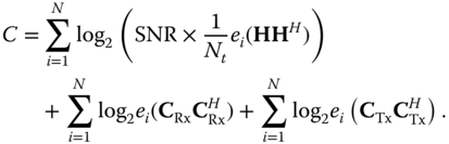
Comparing this result to (2.9), it can be noticed that the last two terms in (2.72) represent the effect of the two MC matrices. MC can enhance the capacity of the MIMO system if the following condition is satisfied,

In other words, the coupling effect will have a positive impact on the channel capacity if the product of the eigenvalues of the two ends MC correlation matrices is larger than one. This has been shown to be the case of closely spaced antennas [148, 150]. However, placing the antennas near to each others results in high SC, which degrades the performance and reduces the MIMO capacity. In the case that antennas were not very close to each other, the product of the eigenvalues of the two ends MC correlation matrices will be smaller than one and MC will then have negative impact on the channel capacity.
2.5.3 Channel Estimation Errors
The ML decoder for MIMO systems as given in (2.3) relies on the knowledge of the channel matrix ![]() at the receiver. Practically, exact channel knowledge at the receiver is not possible due to the presence of AWGN. Therefore, channel estimation algorithm is generally used to obtain an estimate of the channel matrix
at the receiver. Practically, exact channel knowledge at the receiver is not possible due to the presence of AWGN. Therefore, channel estimation algorithm is generally used to obtain an estimate of the channel matrix ![]() [120]. Assuming that
[120]. Assuming that ![]() and
and ![]() are jointly ergodic and stationary processes and assuming that the estimation channel and the estimation error are orthogonal yields
are jointly ergodic and stationary processes and assuming that the estimation channel and the estimation error are orthogonal yields
where ![]() denotes the channel estimation errors (CSEs) with complex Gaussian entries
denotes the channel estimation errors (CSEs) with complex Gaussian entries ![]() . Note that
. Note that ![]() captures the quality of the channel estimation and can be chosen depending on the channel dynamics and estimation methods. In practical MIMO systems, interpolation techniques are generally considered for channel estimation methods. In such methods, the channel is estimated at a specific time or frequency and suitable interpolation methods are used to determine the channel at other points based on channel statistics [151].
captures the quality of the channel estimation and can be chosen depending on the channel dynamics and estimation methods. In practical MIMO systems, interpolation techniques are generally considered for channel estimation methods. In such methods, the channel is estimated at a specific time or frequency and suitable interpolation methods are used to determine the channel at other points based on channel statistics [151].
2.5.3.1 Impact of Channel Estimation Error on the MIMO Capacity
The impact of channel estimation error on the capacity of MIMO systems is discussed in what follows. The MIMO capacity in the presence of channel estimation error can be derived by substituting ![]() and maximizing the mutual information given
and maximizing the mutual information given ![]() , which yields with the lower bound [152]
, which yields with the lower bound [152]

Comparing (2.75) and (2.9) clearly highlights the negative impact of channel estimation error on the MIMO capacity. The SNR decays by a factor of ![]() . For small values of
. For small values of ![]() the impact of CSE is negligible. But for large values, the channel estimation error could deteriorate the achievable capacity significantly.3
the impact of CSE is negligible. But for large values, the channel estimation error could deteriorate the achievable capacity significantly.3