Why XML?

Any popular new software technology has a gee-wizz factor that draws designers to it like so many moths to a flame. Designers are attracted regardless if the new technology is appropriate to the task at hand, often resulting in their demise. So long as a technology is new and interesting, with lots of cryptic acronyms, designers will use it appropriate or not. XML is certainly popular today and has tons of related acronyms, but at first glance XML’s roots as a text document markup language may seem inappropriate for specifying ATE. Why then, exactly, should we use it?

You should use XML because XML has several compelling features that make it ideal to use in the context of synthetic instruments. These compelling features make XML appropriate as a mechanism for describing both synthetic instrument hardware and software and the two working together as a system.

XML has the following distinct advantages in the context of synthetic instrumentation:

ATML

Automated test markup language (ATML) is a cooperative effort by members of the ATE industry to define define a collection of XML schemas that allows ATE and test information to be exchanged in a common format adhering to the XML standard. The work in this book is independent of that effort.

Based on the work I have seen on ATML to date, the XML techniques described in this book are more complimentary to ATML than they are redundant or conflicting. Because of the measurement focus required by synthetic instrumentation descriptions, I address a narrower scope of issues with XML technology than the ATML group is addressing.

I’ll go out on a limb and predict that like many other ATE-related software tools and techniques, ATML will experience gravitation toward the routine, procedural, instrument oriented measurement paradigm. To counterbalance this inevitable gravitation, I would encourage everyone involved with ATML to attempt as much as possible to use the blank slate of XML as an opportunity to do something truly new and better, rather than to simply translate the same old methods into a new syntax.

Why Not SCPI, ATLAS, …?

Before I get into the use of XML, I need to address an objection that I know will be raised by some people. Some folks might think that it would be reasonable to use something else for describing synthetic measurements.

One possibility I’ve heard suggested is SCPI. After all, The Standard Commands for Programmable Instrumentation (SCPI) defines a standard set of commands to control programmable test and measurement devices in instrumentation systems. That seems, at first glance, an appropriate standard. Automated instrumentation developers already know SCPI. In fact, the whole purpose of SCPI was to provide a standardized lingua franca for programmable instrumentation, particularly over the IEEE-488 bus, but over other interfaces (for example, VXI) as well.

No doubt, SCPI can be used quite readily within a synthetic instrumentation system as a way to talk to the individual physical instruments. SCPI has a tree-oriented structure, not unlike XML. It’s also true that SCPI has a related data interchange format (DIF) for recording output data. It’s also certain that it definitely can be used to talk to synthetic instrument systems as a whole and to define interfaces to new synthetic instruments.

Unfortunately, SCPI has certain aspects that make it somewhat problematic for use in describing synthetic instruments, both here in this book, and possibly in a wider context.

First, SCPI provides a standard for an instrument communication interface, not a controllably extensible method for describing synthetic measurements. As such, SCPI really doesn’t exactly fit the bill for the purpose I intend.

Second, listing the set of functions an instrument performs based on the commands it responds to does, to some degree, tell us what measurements can be made. I still could use SCPI to describe measurements, at least SCPI syntax, which is tree oriented, exactly like XML. In this way, I make SCPI do double duty with its role as an interfacing language. However, I believe this would inevitably lead us to a mixed-model, leading us away from an synthetic approach in the design. In its effort to allow for all the diverse functionality of the wide range of automated instrumentation, SCPI provides a rich facility that can be used to describe the interface to virtually any instrument, existing or imagined. That’s not to say it has no limitations. Any practical system must have limitations. Rather, I’m saying that SCPI provides too much flexibility, and thereby allows the designer the ability to design measurements and talk to instruments with any paradigm, synthetic or not.

Automatic Descriptions

XML can be applied practically as a description language in a fully automated context. That is to say it would be practical to start with an XML description of a synthetic instrumentation system, and turn it into a real, high speed instrument using nothing but automated tools.

XML is easy to use with modern compiler tools. Part of this facility stems from the fact that it is possible to express the syntax of XML in Extended Backus-Naur Form (EBNF). If you’ve never heard of EBNF before, don’t be frightened. EBNF is merely a system for describing the valid syntax of a grammar like XML. It’s a way to describe what can and can’t be said in a purely mechanical way.

EBNF comprises a set of rules, called productions. Every production rule describes a specific fragment of syntax. A complete, syntactically valid program or document can be reduced to a single, specific rule, with nothing left over, by repeated application of the production rules. It is possible to express the syntax of XML in Extended Backus-Naur Form, and therefore it is possible to use modern compiler tools that can take EBNF and turn it into compilable high-speed computer codes. Any modern compiler book^[B0] will explain how this works.

Actually, there’s really no need to work at the level of EBNF if you don’t want to. XML has associated with it a large collection of parsers, formatters, and other tools that allow designers to easily attach semantic functionality to XML documents. In most cases, these XML-specific tools are better at doing this than generic compiler tools.

Notwithstanding attempts by some companies to patent encumber various XML applications, thus far XML remains a relatively free and open technology. XML parsing libraries are freely available across many operating systems, and will be found integrated into many development tools. Similarly, there are a wide collection of tools that can be used to write XML. Constructing a GUI, for example, that generates well formed XML is a simple task given all the help available.

Note the statement that XML can be turned into compilable computer code, as compared with interpreted code. Either is possible. The difference between the two is this: Should an XML measurement description be compiled, that implies that all the work of parsing the description and recasting it into a form that can be executed at high speed is accomplished once, up front, before the measurement is ever run. Interpreted code, in contrast, is not processed beforehand. It is processed while the measurement is being run.

Because the processing of interpreted code occurs at measurement time, it has the potential of slowing down the measurement. It’s my opinion that interpreted scripting should be avoided for this reason. Measurement descriptions must be compiled into high-speed, isometrologically optimized state machine descriptions of a canonical map before they are run.

Admittedly, given the ever-increasing speed of computers, this distinction seems less of an issue. Given a fast enough CPU, you can interpret and optimize your measurement every time it runs with no real penalty. Still, I feel that faster CPUs should not be an excuse for slower software or skipping the optimization step. There will always be situations where the maximum possible speed is needed, and you shouldn’t give that capability away for no reason.

Not a Script

The use of XML in automated test applications is nothing new. I have already mentioned the ATML effort. Another application of XML to ATE appears in Johnson and Roselli^[C2], where XML is used as a flexible, portable test script language. Although clever and useful in certain circumstances, I believe “scripting” is an inappropriate use of XML in ATE. XML syntax is clunky for detailed procedural programming; a clunky script language is not what you want from XML in the context of synthetic instrumentation.

Scripting implies sequential execution of a procedural design. Even if object-oriented (OO) techniques are used, and even if the script is compiled, the result is still not as map-oriented and OO as you want; it works at much too low a level; it can’t get optimized effectively. Scripting results in too much freedom, and thereby doesn’t constrain the design approach sufficiently to allow for the best performance.

There are better things to use for scripting than XML. This point is true notwithstanding some of the advantages to the use of XML for scripting that are pointed out by Johnson and Roselli. In scripting, some hierarchical structure is definitely used (subroutines, loop blocks, if-else) but the basic flow is top-down event oriented. For the most part, therefore, XML just dirties up the syntax of what could be a clear procedural script if rendered with a clearer procedural syntax, like one finds in C, Perl, Java, or Forth.

XML is better used as a descriptive language. It shines in its ability to mark things up in a hierarchical or tree structured manner. When you mark up something, like a text document, the markup adds attributes to the text content at the lowest level. It also allows higher level logical structure (paragraphs, tables, sections, chapters, and so on) to be built up with hierarchical layers of markup.

Some applications of XML have what is called mixed content with the hierarchical XML markup intertwined with raw text data at every level. In other cases, there is no content other than structural elements that nest downward at lower levels, possibly with raw data at the very bottom of the hierarchy. In this latter situation, tags and attributes are applied to lower level tags and attributes, down and down till you reach the atoms of content that represent fundamental things that do not apply to anything lower.

XML Basics

Let’s dive right in and look at an example XML document.

Study Example 9-1 and see if you can discern the structure of XML syntax. If you are familiar with HTML, this should look very understandable to you. This is a great advantage of XML, by the way. It’s human readable and leverages the understanding of HTML already possessed by millions of people.

If you aren’t familiar with tagged markup, like HTML, here’s a brief tutorial.

First of all, you need to know that the angle brackets ”<>“are special characters that enclose something called a tag. XML consists of these tags that themselves enclose elements. A start tag begins the enclosed area of text, known as an element, according to the tag name. The element defined by the tag ends with the end tag. An end tag starts with a slash.

One difference between XML and HTML is that in XML, a start tag like <foo> must be followed by an end tag </foo>. The end tag is not optional. However, in XML something called an empty tag is allowed. These have a slash before the closing angle.

Here is an example of a start and end tag enclosing an item:

<foo> this is an item </foo>

This is an empty tag:

<bar/>

Empty tags don’t enclose anything, so they have no associated item. But that doesn’t mean empty tags are, well, “empty.” End tags, like items with no embedded tags, represent a kind of “leaf” of an XML syntax tree.

As with HTML, XML tags may include a list of attributes consisting of an attribute name and an attribute value separated by an equals sign. An example would be <foo bar=“asdf”>, where “bar” is the attribute name, and “asdf” is the attribute value.

For the moment, that’s it. (That wasn’t hard, now was it?) As you can see, XML has extremely simple syntax. In a sense, XML is a way of writing fancy parenthesis to enclose and nest things in a tree structure with handy places to assign attributes at each branching of the tree. There are more things to talk about with regard to XML. I refer you to the many fine books on the subject that are now available^[B6].

Synthetic Measurement Systems and XML

There are many different ways XML fits into the description of a synthetic instrument, but they can basically be divided into these interrelated duties:

The first of these duties is to provide an abstract description of the measurement to be performed. Since synthetic instruments do their work on generic hardware, this first duty is most important. There needs to be a way to describe measurements in a way separate from hardware. XML is exactly that way.

Even though it’s most important, capturing the measurements to be performed is still only part of the picture. The available hardware must be defined so that these hardware resources can be allocated to the measurement tasks at hand. The description of the hardware suite is best done relative to some anticipated fixed yet abstract model so as to structure the description in a way that allows it to be most effectively used. XML can provide exactly this framework.

When the measurement is brought together with the hardware description, the synthetic instrument is generated, loaded into the hardware, and run. The result of the run is a set of measurement data. This resulting data needs to be captured, stored, analyzed, visualized, and possibly augmented or reduced by post processing. Again, XML can serve quite nicely as a data language, encapsulating hierarchical data in a way that can be easily manipulated both by a human and by a computer.

Describing the Measurement with XML

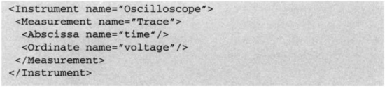
Let’s begin with a simple example in order to show how XML is applied to the task of describing a measurement. Consider a synthetic oscilloscope instrument that measures voltage as a function of time. Here is a simple XML description of the single measurement done by this instrument.

Let’s take a different view of Example 9-2. Figure 9-3 is a diagram of its tree structure.

At the highest level, I have defined an “Instrument” called an Oscilloscope. Enclosed in that instrument is one “Measurement” which I named a “Trace”. The measurement consists of the “time” abscissa and “voltage” ordinate. In Example 9-2, I chose to use empty tags for abscissa and ordinate, with a simple attribute “name=” to give them an identifying title.

I think Example 9-2 is simple enough that you probably understand what I have described using XML, and how I went about it. Admittedly, this a very superficial description. It is also true that I could have used XML in quite different ways to make the same description. I could have structured the description in XML this way instead:

As you can see, what were once attributes have been replaced by a deeper nesting of tags. Is there a reason to prefer one approach over the other? Should a tag attribute be used for “name” rather than a child tag?

In many cases, the answer to this XML style question is unclear. It could be done either way without much difference in this case. One approach would be to use attributes for things that are clearly and tightly associated with the specific tag itself, and no other, rather than something, possibly reusable, that the tag describes or otherwise comprises. In Example 9-3, you should see how the tag <Name> is reused at different levels. Any reusable entity that might apply to different things is probably best a tag rather than an attribute. On the other hand, extremely generic attributes like “name=” are so common that an argument for syntactic simplicity could be made, suggesting that these common things should be attributes, saving us typing, at the sacrifice of complicating reuse somewhat.

There is one situation where there is no decision, where you must use a deeper tag nesting rather than an attribute. Multiple occurrences of an attribute are not permitted. Specifically, it would not be acceptable to make “Abscissa” an attribute of “Measurement” since a measurement could have multiple abscissas. For example, the map description of a image scanner might look like this:

Horizontal and vertical position are the two abscissas, and RGB ordinates describe the color image data. It would not be acceptable to list both abscissas and three ordinates as attributes of the measurement. They must be listed as nested, child tags.

Defining an Instrument

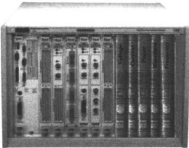
Let’s do another example, a little more worked out to illustrate some further points. This example describes a synthetic instrument that can do two measurements. One called Reflection and the other Transmission. RF Engineers will recognize these as the main measurements of a vector network analyzer, like the Agilent 8510.

The tree structure here is again evident and I have introduced some new nesting elements: Stimulus, Response, and Port.

The <Stimulus> and <Response> elements tells us if the enclosed elements are associated with stimulating the DUT, or measuring some response. Abscissas or ordinates may be defined as canonical only as a a stimulus or only as a response. Thus the stimulus and response nesting will decide what axes in the measurement map must be inverted prior to data acquisition.

The <Port> element is a deceptively simple way to say what physical DUT ports are associated with what parameters of the enclosed elements. Abscissas and ordinate port parameters within are assumed to refer to the listed ports. In Example 9-5, all the abscissas, and the Reflection ordinate refer to the port named input. That name serves to uniquely identify a particular port. It would be assigned in the measurement system description, or possibly as a measurement parameter.

In contrast, the “Gain” ordinate does refer to a particular port; it refers to a <PortGroup>, which are a group of ports referred to collectively. In this case, the port group comprises the ports named input and output. Gain is measured once for this port group. A port group is different than a list of ports, where the ordinate would be measured once for each port in the list. Gain requires two ports to be specified in order to make a single measurement. If you wanted several gain measurements, you would need to give a list of PortGroups.

Ports are, deep down, really just another abscissa. <Port> is defined as an element that contains abscissas and ordinates so as to clarify the parameter passing and grouping issues, but otherwise <Port> will act like any other abscissa. You must set their value explicitly.

You also must say explicitly what the other abscissa values should be for the measurement. Remember, an abscissa is an independent variable, so it needs to be set independently. A Port or an abscissa can be set to a constant value, or it can vary. The “Frequency” abscissa values are an example of an abscissa that varies. It is given as an enumerated list in the first measurement, and by using a <UniformSteps> tag in the second case. Both result in the same actual abscissa points.

The <Unit> element allows us to say what the name of the units are for abscissa and ordinate, as well as giving them an attribute. This allows for automatic unit conversions and tracking.

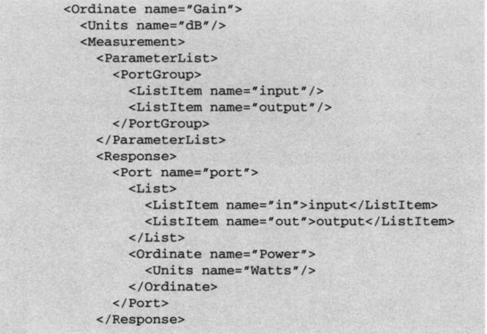
The ordinates specified in Example 9-5 would probably both be compound ordinates in a real instruments. This concept is described in the section titled “Canonical Maps.” It means that there is a calibration strategy specified that will give a schema to rewrite the map into canonical form, with only atomic ordinates specified. Let’s look at what that simple calibration strategy definition might look like for “Gain”.

Calibration Strategy Example

Measurement systems can’t measure gain directly. It’s a relative measurement. Gain can be defined as the ratio of output power to input power of some signal passing through a DUT. The units of gain are customarily expressed in dimensionless decibels (dB), which is 10 log of the power ratio. Unlike gain, power is something that measurement system can often measure directly—it can be a canonical ordinate. If it can measure power canonically, it can break up the compound ordinate “Gain” into two copies of the canonical ordinate “Power”, one measured at the input port and the other measured at the output port of the DUT.

Since input and output power are measured at different ports, I will expand the map with a port abscissa, then specify post processing to collapse the map back down along the port axis.

Study Example 9-6 carefully. There are several interesting elements that deserve some comment. First of all, at the highest level in the tree, I have just an ordinate named “Gain” with units specified just like it was in the network analyzer example. Instead of ending there as it did before, now the ordinate also contains a map for a new (unnamed) internal measurement. The new measurement has no stimulus section, only response. The abscissa of this new measurement is actually the <Port> element (remember I said that ports were really abscissas in disguise). This is a canonical abscissa that specifies how to interact with the DUT. Within the port abscissa, you see that I give an enumerated list of response ports where the system will measure the ordinate, “Power”. This isn’t a port group, it’s a list of ports.

The response port named “input” is really a loopback measurement of stimulus power. I assume that the measurement system hardware allows a loopback measurement of the stimulus at the DUT input. If it doesn’t, then the response port is not canonical over this part of the abscissa domain, and would need to be broken down further, possibly in terms of a stimulus power abscissa. Alternatively, I could define gain itself directly in terms of a stimulus power abscissa, instead of loopback response measured at the DUT input. This alternative approach would not work well on systems that did not have loopback capability. In general, it’s best to say what you really want at the highest level, and break things down till you have what the system can actually do (or at least what some standard set of interface maps can do). Don’t try to make it easy on the system by precanonicalizing based on what hardware you know you have. If you try to do this, you will sacrifice portability.

The <Collapse> element is new. This tells us that the “Port” abscissa is to be collapsed by means of the algebraic equation given. Since there is only one ordinate and it’s a scalar, and the abscissa is an enumerated list, I can use a simple, scalar algebraic equation to perform the collapse. The syntax for the algebraic is given as the simplistic “Power [out]/Power [in]”, which is expresses the calculation of Gain as a ration of two Powers. The “Power” manifold is herein treated as an array indexed by the previously named values “in” and “out” along the axis (named “port”) that I have specified for collapsing.

I call the algebraic syntax simplistic, not because it doesn’t work for this case, and many others, but because one may want to use something more complex here in general. For example, MATLAB syntax could be used, or J, or Perl, or C if you must. You could even link to external code here. Calibration strategy axes collapses need to be able to express all sorts of multidimensional array manipulations, so it would be good to pick something that worked well with that sort of thing.

Here’s an example of a more sophisticated axis collapse one may need. I have assumed power measurement was canonical, but what if it isn’t? If the hardware does not have some fundamental power measuring system like a wattmeter, power would need to be measured by doing a mean square integral of voltage, current, or some other calculation (for example, FFT) based on a block of data. The canonical ordinate in that case might be an array of voltage samples. The map collapse that case would be summing the squares of the data array, perhaps with a primitive as an algebraic expression, perhaps with a full blown script within a <script> element.

Note how units are specified for the result collapse. The units are empty, and therefore dimensionless linear by default, with the conversion to dB left implicit by the fact that the enclosing compound “Gain” ordinate is specified as “dB”. Scale and unit conversions should be performed automagically based on what unit is specified for each axis. This is facilitated by using standard string identifiers for unit names and scales and a separate unit conversion schema that can also be nicely specified in XML.

Another point to notice is the way I introduced identifier references. This is the first time I have used the idea of reference and it represents a watershed in this XML method of describing measurement maps. I have named an axis and some of its elements to facilitate wiring them to the algebraic function. Identifiers and references lead us to the idea of Measurement Map parameters.

Functional Decomposition and Scope

When I defined a compound ordinate like Gain in terms of atomic ordinates, this is really quite similar to the classic functional decomposition that is used with programming languages like C. You start with a complex function, and then partially factor it with several, subroutines. Some of these subfunctions are factored again, and those again, and so on down till you have functions that don’t call any subroutines.¹ Each function in such a decomposition represents a node in a tree much in the same way as the <Measurement> elements represent nodes in the XML tree I have presented for describing measurement maps.

In a classic functional decomposition, each function can have parameters, and optionally return values. This allows us to pass information downward and upward in the functional tree. In the measurement map and calibration strategy schema I have outlined, information flow is implicit between the atoms and the compounds, relying on the fact that their interfaces fit. While it would be nice to believe that this fitting would happen spontaneously on its own, realistically I need a way to specify an interface.

I have used “name=” identifiers to label things within the measurement. Let’s add an explicit <ParameterList> element to say what internal parameters are passed into the measurement from outside. The names associated with these parameters become placeholders for the value passed in. Here’s the calibration strategy map for “Gain” restated with an explicit parameter list.

In addition to their use as parameter labels, I have used element “name=” identifiers as local variables within the measurement, allowing us to refer to specific abscissa values from the <Collapse> block. It would be reasonable to expect that the implied scope of a local identifier is delimited at the <Measurement>, just like the scope of functional parameters.

Measurement Parameters—A Hazard

The <ParameterList> element allows measurements to have parameters. The reason I introduced this capability was because compounds have dependencies on abscissas for calibration strategy. I needed a way to connect this together in an unambiguous way. Using named parameters seems unavoidable here.

Now that they are introduced, measurement parameters have more possible uses that just the atom-compound interface. You may want a way for the test to interface with the measurement, passing down test parameters into a fixed map with variables, rather than rewriting the map with new constants. You can use the <ParameterList> interface for this if you wish.

But do you want to do that? At this point, I start to wonder: When I introduced parameters and variables, aren’t I in danger of turning the XML description of measurements into a real programming language? Isn’t that a bad thing?

Yes, indeed, this is a very dangerous point. Introducing reference in the form of functional parameters and local variables was a watershed for the XML stimulus response measurement map method. It potentially opens Pandora’s box, setting free all the demons that plague anything that threatens to become “real” programming. Until now, everything was pretty and perfect in a context-free way, but parameters and variables seem to threaten that austere beauty, introducing ugly semantic context.

Don’t get me wrong. I’m as much a fan of gnarly-old variable naming and scoping as anyone, but you must remember the goal here is to provide a system that focuses on the measurement with a minimum of computer science arcana. I am dangerously close to introducing a whole bunch of issues that are well understood by programmers, but may alienate nonprogrammers (assuming any are even still reading at this point).

Admittedly I am in danger, but XML itself comes to the rescue. Things are not as bad as they may seem. A Turing-strength programming language has virtually infinite freedom. From this freedom springs most of the problems people have with programming. But XML is different. XML allows freedom, but only in strictly regulated ways permitted by the schema and DTD. The clever folks that invented XML have already seen this hazard and have paved many ways around it.

Therefore, the trick to avoiding these dangers, I believe, has two important aspects:

This trick is easier than it might seem. After all, look at what I have achieved so far with only very limited use of naming and reference. Furthermore, as I have already noted, test engineers are smart people. They will know, intuitively that some measurement parameter is missing and be happy to provide it if asked at the right time. Just don’t turn them into namespace accountants (i.e., programmers). If you do, they will rebel.

Column and Array Data

Column data is the most general data format. It is equivalent to a typical PC spreadsheet data structure. Consider the following example:

Column data tables can represent any number of scalar ordinates and abscissas, including data taken over abscissas that are not separable. If efficiency was not an issue, a column data structure could serve for all measurement map data. That means you can use Excel, or any other spreadsheet format to store map data.

Column data is inefficient in the case of separable abscissa domains. If the abscissa is separable, it is far more efficient, space wise, to store only the factored individual scales for the abscissas rather than the outer product. The ordinate data is stored in ordinary array format. Spreadsheets can store arrays too, but tools that specialize in arrays (J, MATLAB, Mathematica) show their power here. Here’s an example for two abscissas and one ordinate:

The array data format can easily be converted to the column data format, although the reverse is not true, in general.

Self-Documenting Features

Data should always be self-documenting. A flat file of numbers has no meaning once it is separated from the context in which it was acquired. The requirement to self-document derives from good lab practice in general. All abscissa and ordinates must be traceable to type, title, and units. Calibration offsets and other meta-data may also be of importance, so provision should be made for attaching general attribute data to each abscissa or ordinate axis. This should include the capability for “attribute=value” style attributes or the equivalent.

One of the great advantages of object orientation is that if facilitates self-documentation. If the measurement object comprises both the stimulus response measurement map description and the SRMM data, together, and all subsequent report generation and visualization draws from this unified object, you will accumulate a completely self-descriptive entity that paints a complete picture of your measurement. The SRMM object is to the measurement what the TPS is to the test.

Arrays as Elements

Some ordinates are not scalars. For example, the spectra ordinate is a set of spectral power measurements over some domain of frequencies. There fore, column data and outer product array data structures must include the capability of handling arrays as elements. In fact, the most general case allows a data element to be a column data or outer product array. With such a hierarchical format, all possible measurement data can be efficiently and naturally represented.

One way to avoid allowing arrays as elements, but still to permit the same hierarchical freedom, is to allow relations to be defined between data sets. For example, instead of storing a list or array at one location in a table, it could be stored in a totally different table with the two tables linked by a common code number or key. Those of you familiar with relational databases will know that most fields with array contents (other than strings) are stored in separate tables and linked by relations.

SQL Database Concepts and Data Objects

I have been talking about stimulus response measurement map measurement using mathematical terminology from calculus and linear algebra (arrays, vectors, manifolds, functions, mappings). There is, however, an alternative way to conceive SRMM measurements. You can think in database terms (tables, records, fields). The collection of ordinates for a given set of abscissas can be considered a record with the individual abscissas and ordinates representing fields.

Not only can you think about data structures in database terms, you could actually use a SQL database to store measurement maps. This would allow us to conveniently sort and select portions of a larger dataset using standard SQL commands, and the ability to relate other kinds of contextual data for the measurement: date and time, configuration state of the equipment, identifying information from the DUT, and so forth. The idea of using a real database to store measurements has many positive aspects.

The database viewpoint is particularly relevant when arrays are elements. Although linked structures can be built many ways in order to accommodate this kind of element, the methodology of relational database design can help us immensely here.

On the other hand, the creation of a hashed database can be somewhat wasteful for SRMM measurement data because random access to individual records is not a typical requirement. More often, the data is rotated, subdivided, or abstracted in a sequential process for the purpose of visualizing the data with graphs, charts, or plots. Moreover, the raw data itself tends to be very large, making storage efficiency the paramount requirement over efficiency of random access queries and over sorting and searching. Therefore, although the structure of data will readily translate into typical database structures, a simpler, direct indexed data format for acquisition storage can often be a better choice.

HDF

I will sing the praises of XML a lot, but one alternative data format that meets most of the requirements for recording map data is hierarchical data format (HDF). HDF is a multiobject file format standardized and maintained by the National Center for Supercomputing Applications (NCSA) that facilitates the transfer of various types of scientific data between machines and operating systems. Machines currently supported include the HP, Sun, IBM, Macintosh, and ordinary PC computers running most any operating system, even Microsoft Windows. HDF allows self-documenting of data content and easy extensibility for future enhancements or compatibility with other standard formats. HDF includes JAVA and C calling interfaces, and utilities to prepare raw image of data files or for use with other software. The HDF library contains interfaces for storing and retrieving compressed or uncompressed 8-bit and 24-bit raster images with palettes, n-Dimensional scientific data sets and binary tables. An interface is also included that allows arbitrary grouping of other HDF objects.

Any object in an HDF file can have annotations associated with it. There are a number of types of annotations: Labels are assumed to be short strings giving the name of a data object. Descriptions are longer text segments that are useful for giving more in depth information about a data object file annotations are assumed to apply to all of the objects in a single file.

The scientific data set (SDS) is the HDF concept for storing n-dimensional gridded data. The actual data in the dataset can be any of the standard number types: 8-, 16- and 32-bit signed and unsigned integers and 32- and 64-bit floating-point values. In addition, a certain amount of meta-data can be stored with an SDS including:

A more general framework for meta-data within the SDS data model (allowing ‘name = value’ style meta-data) is also possible. There is also allowance for an unlimited dimension in the SDS data-model, making it possible to append planes to an array along one dimension.

HDF is an open, public domain standard. It is matute and well established. It represents a good alternative to XML or SQL databases for the storage and manipulation of synthetic instrument data. The HDF web page is located at http://hdf.ncsa.uiuc.edu/.