
Calibration and Accuracy
Calibration and metrology is an immense topic with numerous aspects. Calibration is particularly vital with respect to synthetic instruments because the SI is the new kid on the block and will be scrutinized carefully by expert and tyro test engineers alike. During this scrutiny, proponents of the new approach want to make sure the evaluations are fair, unbiased, and based on a valid scientific methodology.
Metrology for Marketers and Managers
When somebody decides they want to buy a measurement instrument, the only thing they may know for sure right off the bat is that they want to pay as little as possible for it. But if this was the only specification for a measurement instrument, it’s doubtful anything useful would be purchased.
Sometimes instrument shoppers will specify that the instrument they want to buy should be able to do whatever it does exactly like some old instrument they currently have. But assuredly, if “doing exactly what X does” is the only performance criteria, the system that best performs just like X will be X itself. That’s not likely to be what they wanted, or they wouldn’t be shopping for a replacement for X.
Intelligent people shopping for measurement instruments will think about the measurements the old instruments made and make a list of the measurements they still want. They will present this list of their requirements to various vendors. In this way, they allow suppliers freedom to offer them something other than what they already have. But they don’t want to give the vendors too much freedom, so they need to specify the accuracy they need for the measurements. Customarily they get the accuracy and measurement capabilities from the specifications of X. If the new system meets these abstract specifications gleaned from the specifications of their old system X, they figure they will get something at least as good as X. Sadly, the concepts of measurement and accuracy are often misunderstood, misstated, obfuscated, lied about, or otherwise disguised to the extent that instruments supposedly meeting them end up useless anyway.
For that reason, the most intelligent people will take the time to learn a little about metrology before they go about specifying a measurement system. I feel it’s worthwhile for everyone buying instruments (especially with someone else’s money) to at least know these basics.
It’s beyond the scope of this book to discuss metrology and the scientific method in due detail, but I will include some of the basics in the hopes that it will help some readers cross the line into the smartest group.
Measurand
In the science of metrology, the measurand is the thing you are trying to measure.
Some might want to gild the lily in the sense of Plato’s allegory of the cave and talk about “a true value of the measurand” as something separate, ideal, and unattainable relative to the needle deflections we observe with our human senses. However, metrologists think this “true measurand” terminology is redundant at best. I think it should be sufficient to merely talk about the value of the measurand in the context of a particular measurement method. It’s OK to leave out the “true” adjective, ontological subtleties not withstanding. NIST and other metrology authorities agree with this approach.
The central point is that a measurand is specified in the context of a measurement method. That’s very important. Saying what you want to measure necessarily involves saying how you are going to measure it. It can be meaningless to talk about some parameter you want to measure without specifying a method.1
Unfortunately, it’s sometimes difficult to come up with something that people will agree constitutes a valid description of how a measurement is made without including references to measurement specific hardware. Obviously, this will be a problem when specifying synthetic instruments, instruments that are implemented by software using measurement generic, nonmeasurement-specific hardware.
We, as synthetic instrument designers, want to define measurand this way: Whatever the map measures, that is the measurand. All the context you should need about how a measurement is made is the precise stimulus response measurement map definition of the map in question. In this book, I give you a way to precisely express that in XML. You don’t need to know anything about the hardware. The answer to the question, “How is this measurand measured?” should be, “It’s measured with this SRMM description specification as expressed in this XML document using the resources of the available hardware.”
This answer from a synthetic instrument designer means that in order to decide what it is you are measuring, what you really need to do is exactly specify the maps. You need to decide what the abscissas are, what the ordinates are, how they are sampled, what the calibration strategy is, define any compound ordinates, stipulate the axis ordering, specify what the post processing is, and so on. As you do this, it should become clear that you are really saying “how” the measurement is done, except that the “how” is now broken up and refactored in a way that may seem unfamiliar. It’s object-oriented—not procedural—and that confuses people.
Some may object that fundamentally, someplace, you need to say how you are measuring something the old-fashioned procedural way. For example, someplace you will inescapably get down to an ordinate that measures some fundamental quantity, like mass, time, or voltage. This ordinate will be allocated to a specific measurement asset, loaded a certain way, and applied to the DUT in the context of the abscissa. When you zoom in this close, you will be forced out of the abstraction of the measurement map and have to say how you are measuring that fundamental measurand in a procedural way.
That may be so, but it doesn’t show that there was anything left out specifying the measurement by defining the measurand as a map at the highest object-oriented level. Some details are implicit rather than explicit, yet they are still in there. Some times it’s necessary to zoom in, but you only do that only when you really need to.
Accuracy and Precision
Ironically, the word accuracy as used in common technical discussion is often used inaccurately from a metrology perspective. In fact, the misuse is so widespread and pervasive that it has become the norm in informal technical parlance. Since proper usage of “accuracy” is now in the minority, any attempt to set the record straight may be viewed as nit-picking. People will say, “of course you know what I mean,” referring to their use of the word “accuracy.” But do we know what they mean?
According to CIPM, NIST, and other metrology standard setters, accuracy is the “closeness of the agreement between the result of a measurement and the value of the measurand.” This is a qualitative concept. Accuracy has nothing to do with numbers. It’s OK to say: “This instrument is very accurate.” Or, you can say: “This instrument is more accurate than that instrument.” But when someone says: “The accuracy of this instrument is 0.001 units,” what they mean is unclear.

The word precision, also a qualitative concept, is defined by ISO 3534-1 as “the closeness of agreement between independent test results obtained under stipulated conditions.” This standard sees the concept of precision as encompassing both repeatability and reproducibility (see subsections D.1.1.2 and D.1.1.3) since it defines repeatability as “precision under repeatability conditions,” and reproducibility as “precision under reproducibility conditions.” Nevertheless, precision is often taken to mean simply repeatability.
Both precision and accuracy are qualitative terms. Therefore, to talk quantitatively about the qualitative term accuracy, or, for that matter precision, repeatability, reproducibility, variability, and uncertainty, one needs to use statistical theory. There really is no other choice. Only with rigorous statistical framework supporting you can you make precise quantitative statements like “the standard uncertainty of this measurement is 0.001 units” and have your exact meaning be perfectly clear.
However, if the speaker doesn’t know what standard uncertainty is, there may be a fresh communication problem. You can’t just plug “standard uncertainty” in where you use “accuracy” and expect everything to be hunky-dory. The two terms are very different. For example, increased standard uncertainty means decreased accuracy, so it should be obvious that the two are not interchangeable.
The phrase standard uncertainty has precise quantitative implications. There really is no choice but to learn what the term means if you want to have any chance of using it correctly.
NIST has an excellent reference document online (http://physics.nist.gov/ccu/uncertainty) that quite nicely describes the precise, quantitative meaning of standard uncertainty along with related terms. Anyone interested in making quantitative statements about accuracy should study it as soon as possible.
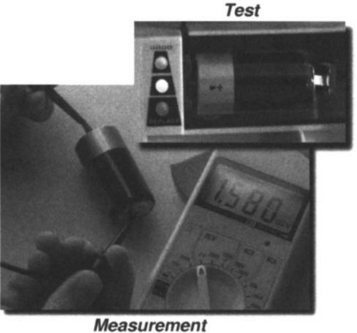
Test versus Measurement
Test and measurement are two words that are often used interchangeably, but they actually are two very different things.
Measurement describes the act of acquiring a numeric value that represents quantitatively some physical aspect of a device. Perhaps it’s a measurement of length, or temperature, or mass, or voltage output of some device. The defining feature of a measurement is it’s numeric result with associated physical units.
A test, in contrast, describes the act of making a decision about some physical aspect of a device. A test has a qualitative result. For example, is the device long enough, cool enough, heavy enough, or does it have enough output? The defining feature here is that a test is the act of answering a question, making a decision, or rendering a pass or fail determination.
The distinction between these two words matters because the methodology for synthetic instrument design that I discuss in this book is primarily related to measurement: how generic hardware can make specific measurements.
Outside the measurement, the process is basically the same for synthetic and nonsynthetic systems. Although it is true that the synthetic instrument, particularly if it’s structure is strictly object-oriented, will likely relate to, or contribute to the test in ways that involve the measurement.2
For example, a synthetic instrument may contribute to how measurements are specified within a test, providing units, ranges, and validation. Or it may support how measurement results are stored, analyzed, and presented within a test, offering formats, analysis, and presentation objects. A synthetic instrument could even go so far as to include methods for performing pass/fail determinations. As such, the instrument has now become a tester, with a standalone ability to perform tests based on the measurements it performs.
Introduction to Calibration
Now I have explained some of the basic concepts of metrology, I can begin to talk about the different aspects of calibration.
Reference Standards
Since instruments need to produce results with true units, the results need to be acquired by means of a measurement process that is traceable to international metrology standards.
Therefore, any synthetic instrument needs standards, possibly several, within it’s architecture. These standards may be for things like frequency, power, attenuation, voltage, time, delay, temperature, and so on. This list is by no means complete. The best standard to use for a particular measurement depends on how that measurement is done.
One calibration philosophy that has certain advantages when applied to synthetic instruments is to employ modular (plug replaceable) standards that allow all the calibration standards in a “sealed rack” instrument to be quickly removed and replaced. This minimizes downtime as the removed standards can be sent as a unit to a calibration lab while the system remains in service with a previously calibrated standards set.
Typical rack-em-stack-em or modular instruments do not use this calibration philosophy. Instead, they calibrate the multiple instruments that comprise the system as individual instruments. The system must be taken out of service to be calibrated. The calibration lab may even be brought to the system in the form of a mobile calibration cart.
Uncertainty Analysis
In order to investigate and predict the uncertainty of a measurement made by a synthetic instrument, the investigator needs to establish the calibration process. Industry practice breaks calibration into three main areas:
Primary calibration is the methodology by which international metrology standards are transferred to components in the system. Operational calibration is the methodology of conducting a measurement and applying calibration information to raw data. Calibration verification is a process, separate from self-test or system functional test (SFT) that seeks to determine, within some defined confidence limits, if the system is currently calibrated. Once the overall calibration methodology is established for the instrument, you can then move on to defining other calibration and accuracy related requirements, like measurement uncertainty, bias, calibration and accuracy analysis, drift, and aging.
Stimulus Calibration
Stimulus calibration is the process by which the stimulus to the DUT is applied at the appropriate value for the measurement. For example, a power supply will stimulate the DUT by applying a voltage. It often is crucial that voltage be exactly correct.
Stimulus calibration is related to inverse maps. The goal of stimulus calibration is to determine how to control the stimulus system so that it generates the required output. In point of fact, the output of the stimulus system (as measured by some response system) is the independent abscissa, and the system needs to determine the dependent control commands (ordinate) that generates that desired output. Since it is reversing cause and effect, this is an inverse map.
There are two common ways to express the intent to set a stimulus to a predetermined value. Either you want the expected value of the stimulus to be at the intended value with some uncertainty expressed by a known probability density. Alternatively, you might want the stimulus to fall within some intended interval of values, with some confidence probability. An example of the first case would be to state that the supply produces an expected 1 volt, with a Gaussian uncertainly of variance 0.01 volt. An example of the second case would be to specify that the stimulus voltage be 1 volt ± 0.01 with a 90% confidence level.
Overall Strategy for Stimulus Calibration
The strategy adopted for stimuli calibration depends entirely on the stimuli involved. In general, however, it represents a good example illustrating how to handle inverse maps and the related concept of stimulus ordinates. I recommend seeking a compromise between knowing the stimuli accurately and the more difficult alternative of controlling the stimuli precisely.
Performing stimulus calibration of a system involves establishing a relationship between the state of the stimulus subsystem and the true absolute stimulus output parameter. Often this is done by creating a calibration map with the following algorithm.
1. Adjust some internal parameter in the stimulus system to a set of arbitrary “state” points (often a grid of approximately uniformly spaced values).
2. Using a calibrated response system, measure the stimulus generated for each of these states.
By means of the calibration map created the measurement can accurately know the stimulus value at each of those states. Calibration strategy algorithms can then invert the map to find the states required to generate any desired stimulus value. Normally this inversion is performed by offline interpolation, but it could be done with a real-time feedback-leveling loop.
Acquisition of an accurate calibration map does not guarantee that stimulus can be controlled with precision. In general, there will be some quantization and repeatability effects that limit the precision of stimulus control to that which the stimulus hardware can achieve, particularly in an open loop configuration.
Using Interpolation to Invert a Map
Interpolation allows the calibration map (or any map, for that matter) to be inverted. Another good reason to use interpolation is to maximize measurement speed by minimizing the number of measurements taken. The question then arises: what is the minimum number of points required for a given degree of accuracy when interpolation is used? There are many possible forms of interpolation: linear, polynomial, least squares, and many others. Often, it is good to choose an interpolating function that matches the function that underlies the real process being approximated. A large body of literature is devoted to this problem[B2].
A favored form of interpolation for continuous functions with continuous derivatives is cubic spline interpolation. Splines have the advantage of passing through specified points and matching the derivatives at those points smoothly. Experience has shown that cubic spline generally provides optimum accuracy in practice when compared with either lower or higher order methods. In this discussion, therefore, I will focus only on cubic spline interpolation as a widely useful practical technique.
The theory of the cubic spline provides the following expression for interpolation error:
in any interior subinterval, [xk, xk+1]
The expression says that the error is proportional to the fourth power of the sample interval, h. Since it’s a fourth power relationship, decreasing the sample interval by a factor of 2 decreases the error by a factor of 16. In practice, this means there is a sharply defined threshold below which it makes no sense to acquire any additional data points.
I can’t overemphasize the importance of this observation. Anyone designing high-speed measurement systems should be aware of the fourth power convergence of the cubic spline interpolation technique, as well as the convergence properties of other, alternative interpolation methods. Why? Because if you aren’t aware of this property, you may design systems that are slower than they need to be, or you may not understand one of the serious issues that affects the speed of your measurements. A fourth power convergence sneaks up on you faster than you might expect.
Often it is the case that instrument systems are designed to take measurements as quickly as possible at some specified accuracy. Basic operation is to make a set of measurements in a vector field over a certain abscissa domain. The time it takes to measure the map is, simplistically, the number of points in the domain manifold multiplied by how long each of them, on average, takes to acquire. Excess points slow the measurement. The best thing to do is to take just as many points as you need to meet your accuracy goal.
Should the convergence error of an interpolation be much smaller than the specified accuracy of the measured points, then meaningless extra data points are being taken and the measurement is slower than it needs to be.
Interpolation Example
A specific example will make this clearer. Consider an output versus input power measurement. In this sort of measurement, the input power into an amplifier is varied as the level of output power is recorded. Input power is the abscissa, output power is the ordinate. Very simple. In numerical simulation, I modeled a saturating amplifier by a sinusoid of amplitude A clipped at magnitude ±1 as is shown in Figure 8-3.

I then computed the exact value of output fundamental power from the Fourier series as a function of amplitude. That result is plotted in Figure 8-4. Notice how the curve bends downward as the amplifier saturates.

Finally, I pretended that I had “measured” the output power ordinate only at 1 dB step intervals of increasing input power. With a cubic spline interpolation, I estimated the points in between those measured steps. The error between the actual values and my interpolated values was tiny. If my interpolated graph were plotted on top of the ideal graph shown in Figure 8-4, it would exactly overlay the ideal graph. To better see how little error there is, look at the difference between the two plots, which is seen in Figure 8-5.

Even at 1 dB steps, the interpolation error is insignificant, peaking at little more than a mere 0.02 dB.
The error convergence properties of the spline method establishes a minimum sampling requirement, beyond which the error rapidly drops into insignificance. Unfortunately, this threshold can’t be established numerically unless the fourth derivative of the function in question is known. In the case of a real-world measurement, one will never know this derivative analytically. It is possible, however, to make a statistical estimate of the next derivative by using so-called Predictor-Corrector and adaptive sampling methods. With these methods, one can estimate where this convergence occurs and adjust the data taking to maximize speed without sacrificing accuracy.
Sampling Interval versus Resolution Confusion
For some reason, people don’t like interpolation. They think it’s not legitimate in some way, that it manufactures data. A synthetic instrument that leverages interpolation for performance gains is somehow cheating.
I think part of the problem one can have with interpolation has to do with a fundamental misunderstanding. There is a lot of confusion between the term “resolution” and the terms “quantization” or “sampling interval,” with many people using the word resolution erroneously to describe quantization in various contexts. In this section, I hope to set the record straight.
Let me begin with two definitions:
Fundamental Definitions
Abscissa Resolution
The minimum interval in an abscissa between which the measurement system when applied to a DUT can produce statistically independent ordinate measurements given a maximum intermeasurement correlation or crosstalk specification.
Abscissa Quantization Interval
The minimum interval in an abscissa between which the measurement system when measuring a DUT can produce unequal ordinate measurements.
The subtle difference between these definitions should be evident. They are similar in some ways. A consequence of this similarity is the confusion between the two that I have often seen. However, despite the similarity in the definitions, the concepts are totally distinct.
Resolution is about independence in ordinate sampling. How close can the system take two samples in abscissa and have the corresponding ordinates be independent. Not just different, but fully independent. Independent, in basic statistical terms, means that the ordinates each can be anything at all within the expected range regardless of what the other was.
Consider a measurement of the temperature versus time of some part in a jet engine. The abscissa is time; ordinate is temperature. How close together in time can the system make two temperature measurements such that one temperature has no influence on the other? Let’s say the range is 0–500°C. The system measures 205.6°C. How long must it wait before taking another measurement such that it can get an ordinate in the 0 to 500 degree range that isn’t influenced by the fact that the temperature was just 205.6? Let’s say we want to measure the engine temperature running, and then cold. How long do we need to wait for it to cool off with the influence of the recent 205.6°C reduced below some acceptable threshold? That’s a question about resolution of measurements.
Obviously, the answer to this question depends on more than just the measurement system. It depends on the thermodynamic characteristics of the DUT. It also depends on some criteria for what it means to “have no influence.” This criteria is the correlation or crosstalk specification I mention in the definition.
The word “resolution” is often used in optics to refer to the resolving power of a telescope or microscope. This form of resolution is measured by specifying how close together, angularly, to image components can fall before they merge into one and become indiscernible based an certain criterion given differently by Rayleigh, Dawes, Abbe, and Sparrow. Angle is the abscissa, image intensity is the ordinate, a criteria is specified, and thus the optics definition of resolution correctly corresponds to the definition I have given.
In contrast, the idea of quantization is not the same thing at all. Abscissa quantization, or sampling interval specifies how close together in abscissa the system can take measurements and possibly have ordinates that are different at all. In the temperature versus time example, how close together in time can you make two potentially different temperature measurements. Perhaps the system has internal processing or the sensor has constraints that prevents measurements from being acquired more often than once per second. If you try to get data sooner than this, you must necessarily get the same answer. If you wait longer than this, the measurement of temperature may well be different to some tiny degree.
How is this related to interpolation? Well, if you understand the difference between abscissa quantization and abscissa resolution, you should be able to see that abscissa quantization can be made arbitrarily small through the use of interpolation. That is to say, you can achieve as fine quantization in abscissa as you want without actually taking any more data or altering the measurement hardware. Abscissa quantization is purely an artifact of processing, and you can choose it to be whatever you want based on the interpolation post-processing you do. You can even change your mind after the measurement and synthesize finer abscissa quantization should you need it.
But you cannot synthesize finer resolution after the measurement. If the ordinate samples are all correlated across the abscissa, you cannot in general make them magically become the same number (or more) uncorrelated samples. Resolution says something immutable about the measurement process. Quantization does not.3
The reason this distinction is of great importance for understanding synthetic instruments is that resolution is a specification given on physical hardware measurement systems that says something about the quality of the hardware. If the meaning of resolution intended by the specification is actually quantization, the specification does not necessarily say anything about the hardware in a synthetic instrument since in many cases the synthetic quantization can be anything you want it to be.
On the other hand, I’m not trying to say quantization is not of any value or importance. Far from it. It is all too often the case that insufficiently fine abscissa quantization is provided despite the fact that it is easy to synthesize more. The reason for this may be that well meaning, scrupulous designers fear being accused of the immorality of interpolation; namely, that they don’t want to make true abscissa resolution seem finer than it is by cheating with interpolation post-processing.
Yet this is misguided thinking. It results in an error in design that is potentially more serious than what it seeks to avoid. Consider the classic “spike” effect visible in uninterpolated FFTs.
If you perform a moderately windowed FFT that results in an impulse-like spectrum, but you fail to zero-pad or use a chirp-Z interpolation to provide quantization finer than the resolution, you will see in Figure 8-6, a deceptive spectral plot that shows a lone spike.

Sometimes the spike sits atop a dome, not unlike an early WWI German spiked war helmet. In all cases, the spike appears suspiciously without sidelobes.
If, however, you use some prudent amount of interpolation, the sin(x)/x structure becomes evident, as you see in Figure 8-7.

Neither plot has more resolution, but I submit that the first plot is misleading, while the second plot is clear and plain. It may be that interpolation gives no additional information in a statistical sense, but it can vastly improve the readability and usefulness of data for humans.
Ordinate Quantization and Precision
Abscissa quantization is probably the most often misnamed as resolution, but ordinate quantization is also sometimes called resolution as well. I prefer to try to keep the matters separate by never speaking of “ordinate resolution,” but rather, to refer to the Precision of an ordinate. Thus, I can also talk about the distinction between ordinate quantization and ordinate precision.
Fundamental Definitions
Ordinate Precision
The minimum statistically significant interval possible between two unequal ordinate measurements by a measurement system when measuring a DUT given a specified confidence level.
Ordinate Quantization Interval
The minimum interval possible between two unequal ordinate measurements by a measurement system when measuring a DUT.
When speaking just about an ordinate in isolation, resolution can be defined as the statistical blurring caused by measurement uncertainty. In that sense, ordinate resolution is a specification of the precision in the ordinate. It’s a parameter that includes repeatability and random noise that prevents us from being able to decide if two different measurement results are different because they are measuring two different true values of the measurand, or because random errors have produced the difference.
One can never know for sure if two unequal measurement results are just caused by dumb luck or if they are “really” different, but one can say with some quantified confidence level that the difference wasn’t a fluke. For example, I might be able to measure a distance to within 1% precision given a confidence level of 99%. That is to say, if two measurements are more than 1% apart from each other, then 99% of the time this difference represents truly different distances. The other 1% of the time they are different based on dumb luck.
This sort of reasoning is related to hypothesis testing and is part of the realm of the science of statistics. If you want to talk quantitatively about measurements, you need to do your statistics homework.[B9]
Ordinate quantization, on the other hand, is the minimum interval between any two different ordinate measurements. It says nothing about the precision of the measurement. All it says is how many digits are recorded. As any elementary science student knows, adding more digits to your answer does not necessarily make your answer any more precise. Only the significant digits count, and those digits represent the true precision of the ordinate.
As with abscissa quantization, ordinates can be quantized more finely after the fact by applying interpolation techniques. Ordinate precision, on the other hand, says something fundamental about the quality of the measurement process and in general cannot be changed merely with post-processing.4
De-Embedding Calibration Objects
Systems often are required to provide for the general concept of de-embedding, which is a generalization of any kind of correction factor applied to an ordinate for the purpose of removing the effects of the physical location of sensors in the measurement. De-embedding effectively moves the measurement from the sensor to some place in the DUT. In support of de-embedding, a synthetic measurement system will accept de-embedding calibration objects from the user or controlling software.

To understand how the de-embedding calibration object is applied, consider the simple case of a single y ordinate measured at a single x abscissa. This is a single real number in some units. The de-embedding calibration object for this measurement specifies how to transform the ordinate from the measured value to the virtual value estimated to exist at some specified measurement point of interest. For example, in measurement of temperature, there may be some known relationship between the temperature at the sensor location, and the temperature at some significant location inside the device being measured. In the case of an integrated circuit die, for example, you may be able to measure or control the electrical power (Watts) into the die, and you may also know the thermal resistance (°C/Watt) between the die and a location where you can measure temperature. The thermal resistance along with the power gives you a de-embedding factor from which you can infer the die temperature.
In general, the de-embedding calibration factor for a particular ordinate will be a function of all the abscissa variables and all the ordinates. Moreover, each ordinate can have a different de-embedding calibration factor. Thus the ordinate de-embedding calibration object is a map, and therefore can have the same data structure as the measurement object itself.
De-Embedding Dimensionality and Interpolation
Although the measurement data from ordinates and the ordinate de-embedding calibration data can be represented by an object with the same overall structure, the de-embedding ordinate calibration object does not need to have exactly the same number of dimensions, dimension lengths, or domain separability as the ordinate measurement object is serves to calibrate.
In the case where the dimensionality is different, it is assumed that the de-embedding calibration factors are constant along those axes. In the case where the dimensions are not equal, it may be necessary to interpolate or extrapolate. How the interpolation and extrapolation is best done depends on the ordinate. In general, linear interpolation and least-squares extrapolation are often appropriate.
Abscissa De-Embedding
De-embedding calibration objects can be provided for abscissas as well. These objects must be available to the system before the abscissa sequence tables are built. They allow stimuli levels to be more accurately and conveniently controlled. As with ordinate de-embedding objects, the application, interpolation, and extrapolation methods are abscissa dependent.
1Not to say that things we have no method for measuring are meaningless, just that it may be meaningless to talk about such things in any quantitative way.
2This isn’t really a character of synthetic instruments. A classical instrument with a proper OO software driver could also contribute to a test in the same way.
3Actually, the statement that you can’t improve abscissa resolution in post processing is false. For certain kinds of measurements, super resolution techniques exist for synthesizing finer abscissa resolution beyond what seems possible given the correlation of the measured data. These techniques trade off ordinate precision (SNR and repeatability) for abscissa resolution. Although not nearly without drawbacks, super resolution techniques have many real-world practical applications and should not be forgotten when abscissa resolution is at issue.[B8]
4Actually, the statement that you can’t improve ordinate precision in post processing is false. For certain kinds of measurements, averaging and decimation techniques exist for synthesizing finer ordinate resolution beyond what seems possible given the random component of the measured data. These techniques trade off abscissa resolution for ordinate precision. In a sense they are the opposite of super resolution techniques that allow us to perform trade-offs in the other direction. Although not nearly without drawbacks, averaging and decimation techniques have many real-world practical applications and should not be forgotten when ordinate precision is at issue.