
Measurement Maps
Large, complex ATE systems are often run by large, complex software systems. The complexity of the software is inevitably a result of the complexity of the system, which is a direct result of the problem solved by the system.
Fortunately, test engineers are really smart people. As such, they have no problem dealing with the complexity of the measurement problem. In fact, the test engineer sees more complexity in the measurement problem than does someone unfamiliar with the details. Because they understand the problem better than anyone else, the test engineer is the best person to figure out exactly what test to run, and exactly how to run it.
Unfortunately, the large, complex software systems that run large complex ATE systems are rarely designed to invite the test engineer to dive in and play. A lot of system-specific software knowledge is required to become productive and avoid breaking things. This specific knowledge has nothing to do with measurements, but rather is related to software architecture and software methodology issues. These issues may be vital from a software perspective, but they really have no direct value to the test engineer. They are pure overhead from their perspective.
Don’t get me wrong. I’m not saying that the typical software found in ATE systems is badly designed. Instead, I’m saying it may have had other priorities—that it is of the wrong design to empower end user participation on a daily basis. The all-too-common problem of measurement-irrelevant software complexity renders big ATE systems inaccessible to the test engineers that need to use them to solve their everyday problems.
This problem is not news to ATE software designers. In fact, ATE software technology has taken step after step in the direction of providing accessible programming interfaces to test engineers. These developments have had varying success in establishing a clear division between the machinery of the software innards, and the machinery of the measurement. Much progress has been made, but none have eliminated the problem completely.
The holy grail of ATE software is a system such that the full complexity of measurement can be expressed by a test engineer with no knowledge of the software innards. The test engineer should be able to design a measurement, from scratch, without being forced to worry about software artifacts, like calling conventions, parameter lists, communications interfaces, and, most of all the programming quirks of the individual instruments.
Much of the arcana that creeps into programming measurement systems is caused by those pesky quirks of specific measurement hardware, and their related configuration issues. Designing a measurement becomes a process of orchestrating a collection of instruments to do what you want them to do. This is an inherently complex task because each instrument has its own set of capabilities, expressed in nonuniform ways. Admittedly, things like SCPI and VXI plug and play go a long way toward unifying the look of a collection of unique instruments, but you still have a collection of unique instruments, albeit “smoothed over.”
This is why synthetic instrumentation is such a breakthrough for software accessibility. For the first time, designers can define a measurement application programming interface (API) that is just about measurements and only about measurements. The irrelevant machinery is hidden. The test engineer sees a totally measurement-oriented interface through which they can express whatever it is about the measurement that needs to be expressed.
In this book, I introduce the stimulus response measurement map (SRMM) model of measurements and XML-based SRMM measurement definitions as one way to define measurements in a synthetic measurement system that stays focused 100% on the measurements. I wouldn’t claim that my approach is the only possible approach, but I submit that it provides a proper foundation for ATE application software that is fully and exclusively based on the measurement, and thereby facilitates the construction of user interfaces that spare the test engineer from irrelevant considerations outside the measurement.
Measurement Abstraction
It is a sad irony that focusing on the measurement for the purpose of making life simple for the test engineer leads to abstraction, and a new abstraction is never simple for anyone to accept at first. I would go so far as to say that the most formidable human problems facing the introduction of synthetic instrument design concepts in real-world applications is the fact that synthetic instrumentation embodies an abstract model of measurements. When people are accustomed to dealing with concrete things (for example, a specific set of instruments that they use to make a specific measurement), it becomes very difficult for them to let go of this conception of things and try to imagine any other way to accomplish the measurement.
This fact about human nature is why virtual instruments are so popular. With virtual instruments, you can imagine that your favorite old instruments are still being used to make your measurement. You can have comforting little virtual knobs on cute virtual front panels constituting your virtual rack of virtual instruments. This collection of instruments are then programmed in a quite familiar manner that mimics the way a corresponding set of physical instruments would be applied to do the measurement.
But actually, if you want to measure something, Yogi Berra might say that all you really need is a thing that measures what you want to measure. If you want to measure A and B vs. C and D, you need an (A,B) = f(C,D) measuring instrument, an AB vs. CD meter, so to speak. Nothing else is really the “right” thing. Yes, maybe you have always measured A and B separately as functions of C and D and stitched it together, but fundamentally what you really want to do (if you don’t mind me putting words in your mouth) is measure the AB vector over the CD manifold1.
This idea becomes crucial when C and D are not separable. A function of several variables:
is separable if it can be expressed as a product of functions of the individual variables.
Here’s an example: Suppose you have an ultrasonic transducer. You would like to measure its response versus frequency and its response versus signal input level. These two measurements may not be separable. You could vary input level and plot output at some fixed frequency. Then you could vary frequency and plot output at some fixed input level. If the response was separable, you could then multiply those two functions and have the whole thing.
But it may be the case that the shape of the frequency response curve changes at different power levels. It may also be the case the power transfer curve is shaped differently at different frequencies. You really need to measure the response over the joint domain manifold of frequency response and power response to fully characterize the sensor.
Figure 6-1 is an example of a manifold f(x,y) that isn’t separable.

Synthetic instrumentation approaches don’t yield their biggest payoff unless you are willing to think about measurements themselves, as pure measurements, especially multidimensional measurements. You need to divorce your thought from particular instrumentation used to make the measurements and think only about what you want to measure, in and of itself. Failing to do this will inevitably shift the focus from the measurement to the instrument being used and result in the introduction of myriad irrelevant and extraneous considerations that would not otherwise appear.
To the end of attempting to get everyone thinking about measurements abstractly, the following section attempts to introduce some vocabulary that does not shackle us to instrument-specific ideas. The vocabulary is based on mathematical concepts that, for the most part, are studied by teenagers in high school.
General Measurements
In a synthetic instrument, measurements are performed by software running on generic hardware. Ideally, this software is completely flexible. Any sort of measurement is possible to define, so long as it falls within the capabilities of the hardware. Unfortunately, if measurements are flexible without limit, one is wandering without guideposts in this total freedom. The system can do anything, so there’s no structure to provide a handle on what can be accomplished.
For example, there is no finite set of distinct measurement parameters that fully describe the required inputs to all these possible measurements. Moreover, there is no possible universal parameter format, type, or structure that can cover all cases. Similarly, in general there is no standard data type to cover all possible measurement results. Nor is there a finite and standard calibration set that can be applied to relate these arbitrary measurements to physical units.
It should be clear, therefore, that some sort of structure must be imposed on this vast abstract possibility in order for our finite human resources to be applied. One type of structure is the virtual instrument structure. This introduces the accustomed structure of everyday instrumentation in order to make our options reasonably finite.
But virtual instruments are not unlike the way stops on a church organ mimic classic musical instruments. The organ can synthesize various classic instruments, but if you wanted something else not in the set of organ stops—something new—you couldn’t have it. This isn’t because of any inherent limitation in the organ, but rather because of a limitation in the model used to parameterize and limit what the church organ can be asked to synthesize.
What is needed is a structure on possible measurements that is limiting enough to result in a tractable system design, but generic enough to allow the full range of possibilities. Returning to the organ metaphor, introduce the idea of a Fourier series, and allow organ stops to be specified as Fourier coefficients. Now the goal is reached. The Fourier series provides a handy and compact structure without introducing practical limitations. The full freedom of synthesizing any past instrument lives along with the possibility of synthesizing future instruments.
Abscissas and Ordinates
I will now propose a system for describing measurements that is free of specific instrumentation focus, and thereby does not require reference to virtual instruments, or any other legacy crutch. It is compactly and usefully structured, but the full freedom of synthesizing any past instrument lives along with the possibility of synthesizing future instruments.
In this system, I consider only the subset of all possible measurements that I call stimulus response measurement map (SRMM) measurements. I will show that with this conception, a uniform format for parameters, data, and calibration is possible. This has far-reaching significance because the broad class of SRMM measurements comprises all the typical measurements made with conventional instrumentation, as well as much of what is possible to do with any instrumentation.
The Measurement Function
SRMM measurements are based on the concept of an abscissa and an ordinate. You may remember these words from high school. If you remember what they mean, you are ahead of the game because I will not alter their meaning in any fundamental way. All I will do is to observe the fact that these concepts represent a measurement in a generalized manner first elucidated by Isaac Newton.
The variable x represents the abscissa and y represents the ordinate. The function f relates the two. If you don’t like the words abscissa and ordinate, perhaps you might prefer the alternative: independent variable (abscissa), and dependent variable (ordinate). Or maybe you just like x and y. Some purists think that abscissa and ordinate should be reserved strictly for the case of a two-dimensional plot. Fearless of the wrath of the math gods, I will use abscissa and ordinate terms to refer to independent and dependent variables regardless of the dimensionality of each.
In a sense, the function f represents the measurement process, with the abscissa representing the state of things, or possibly some imposed state (stimulus) and the ordinate representing the measured or observed response. Mathematically, a function is defined by specifying its ordinate for every possible abscissa over some domain. In the case of a discretely sampled domain, a function can be defined by simply enumerating the ordinates in a table. For example:
| x | y |
| 1 | 10.0 |
| 2 | 10.41 |
| 3 | 10.73 |
| 4 | 20.0 |
| Time (hr) | Temp (°C) |
| 1 | 10.0 |
| 2 | 10.41 |
| 3 | 10.73 |
| 4 | 20.0 |
Not all possible tables define valid measurement functions. The definition of a function requires that there be one and only one value of y for any value of x. Therefore, a table that listed x = 2 several times with different values of y would not define a function. Analogously, in the context of a measurement, this requirement translates into demanding that the system produce one and only one measurement for each value of abscissa. Normally, such a requirement isn’t a problem. In the case of inverse maps, however, it may become a sticking point.
Canonical Ordinate Algorithms
Much of the technique of measurement in a synthetic instrument is encapsulated in so-called canonical ordinate algorithms. These algorithms generally represent the crux of the measurement issues—the down and dirty business of finally getting a number.
Canonical ordinate algorithms, as such, are not concerned with the context of the measurement, abscissa rastering, or data structures. These other issues have been abstracted away and are handled by other algorithms and data structures in the stimulus response measurement map model.
Multidimensional Measurements
Functions can have more than one abscissa. In such a case, the domain is a multidimensional manifold or, more loosely, surface. If, for example there are two abscissas, u and v, the the function of two variables:
can be defined over a discretely sampled two-dimensional (u,v) domain with a table, thus:>| u | v | y |
| 1 | 4 | 5 |
| 1 | 5 | 6 |
| 2 | 4 | 6 |
| 2 | 5 | 7 |
Once again, for this table to define a function, there must be one and only one value of y for each unique (u,v) pair.
Domains
Note the interesting pattern that the (u,v) abscissas make. It should be clear that this pattern is formed with an outer, or cartesian, product of two uniformly sampled abscissas, [1,2] and [4,5]. This produces every possible combination of the individual abscissa values. An outer product can also be visualized as a table. Here is the outer product table that produced the above abscissa pairs:
| uv | 4 | 5 |
| 1 | (1,4) | (1,5) |
| 2 | (2,4) | (2,5) |
Not all discretely sampled multidimensional domains can be represented as outer products; however, those domains that can be represented with an outer product, I call separable. The advantage of the separable property of a domain is that it can be represented very compactly by the sampling grids of the individual abscissas. The abscissa pairs in the outer product do not need to be stored explicitly after the measurement. Fortunately, separable domains constitute, in large measure, the kinds of measurement domains people like to use. There are, however, some restricted special cases of nonseparable domains that are of interest. For example, consider the measurement table:
| u | v | y |
| 1 | 2 | 3 |
| 2 | 3 | 5 |
| 3 | 4 | 7 |
| 4 | 5 | 9 |
I call this kind of domain locked. There is a fixed difference between the u and v value. In many measurements, abscissas are locked in ways analogous to this. A received frequency might be locked to a transmit frequency, a response port may be relative to a stimulus port, there are many examples of abscissa locking.
The final kind of nonseparable domain that is commonly used for measurements is called banded. In such a domain, one abscissa varies independently, and the other varies in a restricted range around the first. A banded domain can be represented as a diagonal subset of the outer product of a separable domain. For example, the domain table:

| u | v | y |
| 1 | 1 | 4 |
| 1 | 2 | 9 |
| 2 | 1 | 9 |
| 2 | 2 | 16 |
| 2 | 3 | 25 |
| 3 | 2 | 25 |
| 3 | 3 | 36 |
| 3 | 4 | 49 |
| 4 | 3 | 49 |
| 4 | 4 | 64 |
Banded domains are useful for measurements that explore a region in a two-dimensional domain of some ordinate where stimuli or abscissas vary in a coordinated, but not strictly locked, manner.
Measurement Maps
In a measurement process, it is often convenient to make several different ordinate measurements at a given abscissa point. Moreover, the ordinates may range over a multidimensional domain manifold with several independent abscissas. Therefore, to represent measurements, I need to generalize one-step further from a scalar function of several variables to vector-valued function of several variables, a so-called measurement map.

Although the concept of a vector field or multidimensional mapping comes from mathematics and therefore evokes latent math anxiety in people, I’m not really saying anything deeply difficult here. Oddly, if I talk separately about measurement data as multidimensional, or the multidimensional domain manifold over which the data is taken, people seem to understand that just fine. It’s when I put them together into a vector valued function of a domain manifold, in a simple word, a map, that the eyes glaze and the knuckles whiten.
But consider, for example, an X-Y positioner moving an image sensor around. A common flatbed scanner like you have on your PC is an example. Clearly the position of the sensor is a two-dimensional thing. And if I talked about an X-Y-Z positioner, possibly with some theta angular rotation of the sensor, the resulting four-dimensional set of variables isn’t very hard to take. Any number of independent variables are easy to understand.
When the scanner acquires color image data in red, green, and blue color dimensions, it establishes a relationship between the image intensity vector in RGB space, and the X-Y spatial location. This relationship is what I call a measurement map, and the data itself is measurement map data. (See Figure 6-3.)

A measurement map is the relationship between a set of independent variables, and a set of dependent variables. It’s how the elements of one table or spreadsheet relates to another table or spreadsheet. That’s it. Nothing more tricky than that.
Ports and Modes
I’ve talked endlessly about measurements. How do these relate to a DUT? What is the link between the two? A bridging concept that I use to relate a DUT to its measurement is the concept of a port. A port is a plane of interaction between the measurement system and the DUT—a precisely specified data interface between the signal conditioner and the DUT. Often it is a physical cable interface to a sensor or a connector on the DUT, but it might be an abstract plane in space. It depends on what you are measuring and how.
Many schemes have been developed for managing ports and linking logical ports to the real physical wiring interfaces, registers, or commands they represent. These schemes tend to be proprietary and associated with particular measurement systems. Others are more generic. I will present a sketch of a minimal scheme in the section titled “Describing the Measurement System with XML” that uses XML syntax.
Ports can have many attributes, but foremost is if the port is an input to the DUT, or if it is an output from the DUT. This will determine if the measurement system applies a stimulus to the DUT at a given port, or measures a response.
In my model of a synthetic measurement system, ports must be associated with physical point or planes, and must be categorized as either stimulus or response. They can’t be both, or neither, although it is certainly possible to define two ports, one stimulus and one response that both connect to the same place, or no place.
Ports are a logical concept, but ultimately they connect to the real world. Stimulus ports are, ultimately, controlled by a register that is written or a command that is sent; response ports are likewise wired to a register that is read or a command that is received.
The port is not the only bridging concept that links from the measurement to the hardware. A mode denotes states of the system itself independent of its physical interfaces.
The distinction between ports and modes is a fuzzy one. Perhaps the signal conditioner has two separate physical interfaces: One through an amplifier and one direct, with a switch internal to the conditioner selecting between them. I might call that switch a mode switch. On the other hand, suppose these two conditioner ports are connected to different DUT ports. Maybe then the switch is really a port switch. But what if the switch matrix outside the conditioner is able to route either of these signal-conditioning interfaces to the same or different interfaces on the DUT. Now it may be unclear if the gain selection switch should be considered a port or a mode.

It might be argued that implementing a mode by means of a physical interface, mixing the two concepts of mode and port, might be considered a hardware design mistake in the same way as a GOTO statement is considered, by some, to be a mistake in software design. This would be true if there were no other considerations, but the reason hardware is designed a certain way (or software, for that matter) is frequently based on the optimization of certain aspects of performance, along with considerations of safety, cost, reliability, and so forth. There may be good reasons to use separate physical interfaces for different modes in a signal conditioner that override any paradigm purity considerations.
A common voltmeter is a good example, where the high-voltage measurement input is often a different interface than the normal, low-voltage input. This is done in order to reduce the chance of damaging the low-voltage circuitry with an accidental high-voltage input, as well as eliminating the need for an expensive high-voltage switch in the meter.
In general, it is wise to distinguish and separate modes from ports as much as possible. In a well-designed SMS, there will be a site configuration document and associated software layer that can disentangle many of these overlaps between ports and modes.
DUT Modes as Abscissas
Quite often, the measurement system is called upon to control the DUT. For example, suppose the DUT is a radio receiver. A reasonable measurement of interest might be the sensitivity of that radio receiver. But the sensitivity of a radio depends on its settings: where it is tuned in the band, if it’s set to AM or FM, and so on. If the radio can be controlled by a measurement system, we can ask that system to measure the radio’s sensitivity as a function of tuning and other mode settings on the radio.
When a DUT is controlled by the measurement system during testing, the DUT modes become abscissas. Even though they are not part of the measurement system, per se, they represent an independent variable just as much as any other port, mode, or abscissa within the control of the measurement system.
Ports as Abscissas
Ports are related to the measurement map in an essential way. Each abscissa and ordinate in a stimulus response measurement map must be associated with a port. Also, one or more ports may be defined as port abscissas. It’s best to think of ports as a special kind of abscissa (a child class) that behaves for the most part exactly like an abscissa, but has the additional ability to bind other abscissas and ordinates to a physical measurement port.
In this way, all the machinery developed to sample abscissa domains becomes available to select the port used for each measurement. This approach makes a lot of sense because abscissas define the independent variables in the measurement; they define what is controlled and specified; they establish the domain over which the ordinate is measured. Similarly, modes are also sensible to make into abscissas as they, too, represent the independent context of an ordinate.
If you make port and mode selection through abscissas, it’s clear that these port or mode abscissas may apply either to stimulus, response, or any combination thereof. This point matters most when specifying a calibration strategy that may introduce new calibration abscissas, or otherwise transform the map from what the user specified to what the machine can do.
Map Manipulations
If you have followed me so far, you should see that the description of a measurement and the results of measurements are mappings. Using the stimulus response measurement map model of measurements allows us to see exactly what aspects of each particular measurement are unique to that measurement, and what parts are generic aspects. Looking at the map as a whole allows us to see beyond the particular list of abscissas and ordinates associated with a test and focus on the measurement itself. This measurement focus leads inevitably to a compact implementation as a synthetic instrument.
In regards to abscissas, in the common case of a separable domain, the process of applying stimuli to a device can be reduced to defining the individual abscissa scales. With the addition of banded and locked domains, all usual domain cases are comprised by a small set with compact descriptions.
There is a distinction between a map description and the map data itself. The map description is present before the measurement is made. The map data is acquired after the measurement is made. Together they represent a fully documented measurement map. Often I will discuss the two collectively using just the one word map. In cases where the distinction is relevant, I will explicitly specify map description or map data.
Maps are more than just a way to define measurements and record the results of measurements. Maps can change. They can be processed and manipulated both before the measurement and after the measurement in ways that are isometrological—manipulations that do not affect what is ultimately measured. In fact, they must be processed and manipulated isometrologically in order to apply to many common measurements, particularly relative measurements, or measurements that include a calibration ordinate. This isometrologic manipulation process is called canonicalization. It is described in detail in the section titled “Canonical Maps” and it is the paramount benefit of the Stimulus response measurement map viewpoint.
Maps can be interpreted (with some restrictions) as a multidimensional entity, as a manifold themselves. As such, all the concepts associated with manipulating objects in space work as tools for manipulating maps. For example, you might take a slice through a particular plane. A slicing action represents holding the value of some variable constant, either an abscissa or ordinate. Imagine a measurement of an amplifier gain and power supply drain as a function of input power and input frequency. Maybe you might like the gain versus frequency at constant power supply current. That would be a slicing operation. Slicing operations usually require interpolation because the plane that slices through the data may fall between measured or controlled points.
Processing may also rotate the map. This may be done to reorder the axes, or perhaps to remove dependencies between axes—to orthogonalize axes. An example of orthogonalizing would be a DUT that has two inputs and two outputs. Both inputs affect both outputs, but the inputs affect the outputs in different ways. Imagine, for example, the hot and cold knobs on your sink. They control the temperature and flow rate of the water out of the spigot. Two abscissas, two ordinates. There is an interaction between the two. Turning one knob changes both the flow and the temperature. Maybe you would like to know how to control just the temperature at a constant flow, or the flow at constant temperature. That is the process of orthogonalization applied to measurements. In this case, it involved finding a rotation transformation to apply that orthogonalizes the abscissas.
When rotating more than just the abscissas, the rotation can be interpreted as an inversion of the map. For example, if you have a map y = f(x) and you find a function g that exchanges y for x, allowing you to get x = g(y), then you have rotated and flipped the x-y plane. That is to say, you have rotated abscissas and ordinates together, as one unit. Inversions, like slicing, require interpolation in order to make the new abscissa fall on nice, uniformly gridded points.

Sometimes it’s necessary to flatten a map. This process removes an abscissa or ordinate. Calibration is often accompanied by flattening. For example, suppose you are measuring the gain of an amplifier. You may do that by measuring its input power, then its output power, then dividing the two, yielding gain. After the division, if you no longer want input and output power, you can flatten the map data manifold by combining two of its dimensions with a calculation. In that case, I call gain a calculated ordinate as compared to the directly measured ordinates of input and output power.
Maybe you want to expand (or maybe better would be thicken) the map data with the gain calculation result, keeping input and output power in place. This is fine too. Expanding is the dual of flattening. It’s common to add new dimensions to map data during post-processing with additional calculated results; it’s also common to add them in preprocessing to include calibration ordinates or abscissas. Sometimes these expansions are paired with their dual, a flattening, on the opposite side of the data acquisition.
An alternative to expanding and flattening is to make a child map. When creating a child map, it is generated from one or more parent maps by a calculation. It’s a good idea to maintain a link between child and parent so that later you can figure out what the calculated data was based on. This is often done in a nested or hierarchical tree-like manner that can easily be expressed in XML or HDF.
Other dual-pair manipulations that are useful are rastering and raveling. Both of these ideas are implicit in the way domains manifolds are sampled. Normally, where there is more than one abscissa, the abscissa is sampled in raster order. That is to say, one of the axis is sampled so as to vary fastest in an innermost loop with the other axes held constant. Then, once the innermost abscissa is completely sampled across its domain, the next innermost abscissa is incremented to its next domain sample point, and then the innermost repeats its scan. Thus, all the axes are sampled through their ranges in this way.
An alternative to rastering is to ravel the abscissa points in some other order. All points are still sampled, but the samples are ordered differently. Normally, the order in which the abscissa set is sampled does not affect the measurement, but when hysteresis is present, or when certain axes are slow and others are fast to measure, the ravel or raster order can be essential to the success of the measurement.
All these manipulation techniques, and more, can be used on measurement maps. They can be used individually, or in combination. What is less obvious that should be emphasized is that they can also be used either on map data, or on map descriptions. This may be surprising to you if you had been thinking of all these cutting, flattening, and interpolation operations as after-the-fact post-processing of map data.
Operations on map descriptions are performed differently than operations on map data, that is true. But the same set of techniques are generally available. One can expand the map description to include extra abscissas or ordinates before the measurement; similarly, one can interpolate, invert, or otherwise reshape.
Consider the gain measurement example again, beginning with a map description that gives gain as an ordinate. One of the pre-processing steps might be to expand the map into canonical form with an atomic input power and output power ordinate.2 This would be done by canonicalization so that during post processing the operation could be reversed, yielding gain.
In fact, it is a general rule that calibration strategy considerations often will required a transform of the map description prior to the measurement. Any time you make a relative measurement, for example, the relative ordinate you want to measure must be split into multiple measurements, which are divided or subtracted or otherwise combined through some calculation to compute the desired computed ordinate.
Problems with Hysteresis
There is great advantage to thinking about maps as entities that can be manipulated by standard operations, as if the maps were made of modeling clay or tinker toys. In many cases, clever manipulation yields great efficiency in measurement activities, giving us faster, better, and cheaper measurements.
Unfortunately, there are metrologic issues regarding accuracy that must be addressed. One of these issues is interpolation, relied on by many map manipulation techniques. Issues with interpolation are discussed elsewhere in this book. In this section, I will discuss another key issue that hurts the ability to manipulate maps. That issue is hysteresis.
It is a fact that many DUTs have memory. That means that the results of one measurement on the DUT depends on what measurements have been made previously. For example, temperature is an issue for many devices, and making measurements can alter the temperature of the device, thereby changing measurement results. Many other examples exist of this phenomenon.
As a consequence of hysteresis, the order in which measurements are taken can be crucial. In situations where hysteresis is an issue, the cutting, slicing, and rotating manipulations that are performed on some maps may not be performed arbitrarily without risking significant loss of accuracy.
There is a distinction between memoryless devices and devices that can exhibit hysteresis. When faced with a DUT that has memory, there is no alternative but to evaluate what measurements are being taken, at what speed, over what duration, and what effect on the DUT will be retained and affect future measurements. Only once these considerations have been evaluated, can appropriate constraints be applied on map manipulation so as to avoid any loss of accuracy.
Stimulus and Response
Stimulus and response are interactions with a device under test (DUT). Don’t make the mistake of thinking an abscissa is a stimulus, or a response is an ordinate. An abscissa is an independent variable that you set. It establishes a context for a measurement. The ordinate is that measurement. Yes, an abscissa is ordinarily related to setting a DUT stimulus because the stimulus plays a major role in setting context. Similarly, a DUT response is ordinarily related to an ordinate, because the fundamental idea of test and measurement is to measure the DUT response to some stimulus. These relationships are typically true, but not always.
In fact, it’s quite common that an ordinate is associated with measuring the applied stimulus so as to verify that the correct stimulus was applied during the measurement. Later, in post processing, the stimulus ordinate may be isometrologically transformed into an abscissa, but it starts life very much as an ordinate.
Another example would be in a system that analyzes modulated or coded responses from a DUT. An abscissa in such a system might be receiver frequency or subcarrier number or any of a number of possible response attributes that independently set the context for the dependent ordinate.
For this reason, there must be a mechanism to explicitly associate the axes in a map to a stimulus or response.
Inverse Maps
A surprisingly helpful concept is the idea of an inverse map. Consider a two-port device under test, like an amplifier. The measurement system provides an input stimulus, and measures the output response. With this sort of setup, you can measure a map like gain versus input power and frequency.
Now, suppose somebody wanted to know what input power was required to hold the output power of the device constant at some fixed level versus frequency. In essence, they want to measure a stimulus or cause (input power, frequency) that results in a certain response or effect (output power).
This sort of case is another example that demonstrates not all ordinate measurements are of responses. Sometimes we try to find out what stimulus causes a certain specified effect in the response.
Assuming we are in a causal thermodynamic universe where effects follow causes in time, it won’t work to choose the effect first, and then see what cause “happens.” All you can do is to try some causes and record their effects. Afterward, on paper, you can invert cause and effect to see what causes would be needed given certain desired effects.
This reversal of cause and effect is an inverse map. When the test engineer specifies a map that has reversed cause and effect, the calibration strategy must be to invert the map so that it can actually be measured forward in time.
One way to achieve map inversion is to do a measurement to acquire a causal, noninverted or natural map, and then in post processing invert the map mathematically, resampling and interpolating as needed.
But is there any way to reverse cause and effect without inverting a map after the fact? Is there some way to apply an effect, and measure a cause?
Surprisingly, in some cases, the answer is yes!
Let’s return to the case of the amplifier. I want to know what input power, versus frequency, will keep the output of the amplifier at some constant output power. Suppose I constructed a feedback loop in my measurement algorithm. This loop would implement a goal-seeking algorithm that would adjust the input power so as to keep the output constant. With this loop in place, I could vary the frequency and measure the input cause that produces the constant, specified effect. Consider, as another example, the square root circuit in Figure 6-6 that works using this same principle of inversion performed by a feedback loop.

“Cheater!” you shout. I didn’t reverse the flow of time. Within the feedback loop, minuscule accidental errors in stimulus cause deviations in the output that result in corrections of the stimulus. So the map really still does get inverted, in a sense. Well, maybe you’re right. But it is certainly true that feedback loops and adaptive systems seem to invert cause and effect, and they thereby represent a powerful tool for inverting measurement maps coincident with the moment of measurement itself.
Accuracy Advantages of Inverse Maps
As a general rule, a measurement designer should always consider the possibility of inverting cause and effect in her measurement, measuring something backward, and afterward inverting the map. This possibility should be compared with doing the measurement the forward way. In many cases, the inverted method leads to more accuracy, simpler hardware, or both.
A classic example of the advantage of inversion is when calibrating a variable attenuator. A variable attenuator is a device that takes an input signal and reduces its amplitude by some selectable amount. These attenuators are calibrated by setting them to all their states and measuring the reduced output level relative to the input. The forward way to accomplish this measurement would be to stimulate the DUT with a fixed input, vary the setting of the DUT as an abscissa, and acquire the output level as an ordinate.
Unfortunately, with attenuators that work over a wide range, this approach may be quite inaccurate and slow, especially for when the attenuation setting is high resulting in a very small response. When he realizes that his response system sensitivity is inadequate to the task, a test designer who hasn’t read this book might decide that he needs more sensitive hardware in the response system.
The right thing to do is to consider an inverse map. Fix the response out of the DUT and allow the stimulus to be the ordinate. In doing that, the response system can work at a level that is comfortable and accurate, and the requirement for wide dynamic range is shifted to the stimulus system, which may already have that capability since it is far easier to generate a wide range of levels accurately than it is to measure them.
Sadly, if there is no software support in the synthetic measurement system for inverse maps, the test designer may see the hardware solution as easier to implement. This illustrates a common mistake in the development of synthetic instrumentation that I discuss elsewhere in the boot: exclusively using hardware to fix problems.
Problems with Inverse Maps
Inverse maps are not without drawbacks. Two that I will mention here are the problem with inverse function branches, and the problem of adaptive stability.
After inversion, a map may not still be a map. That is to say, the result may not be a function. There may be more than one value possible for an ordinate at a given abscissa point. The alternative values are called branches of the inverse map.
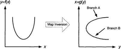
The right branch to pick for the inverse may not be immediately clear. One option is to split the map and carry each branch forward separately in a collection of maps. In other cases, constraints and defaults provide a way to pick the right branch.
Another difficulty sometimes faced by inverse maps is the problem of stability. When map inversion is performed by real-time adaptive algorithms, the feedback loop within that algorithm may oscillate. If the system relies on such an adaptive loop to perform map inversion, instability in that loop would be disastrous to the accuracy of the data. Fortunately, there is a large body of theory regarding the stability of feedback loops, and there is much practical advice about how to go about fixing unstable loops.
Calibration Strategy and Map Manipulations
Why did I bother to create the stimulus response measurement map model of measurements? What good is it, really? Maybe it seems like an interesting way to describe measurements, but is there any big payoff? These are good questions. It may not be obvious why any of the math stuff is worth the trouble. Abscissas are just fancy loops. Ordinates are measurement subroutines. Yes, I see how this ties data together with the measurement in a neat package. That’s nice. But is there a bigger payoff?
While I have already pointed out the many small payoffs that derive from the use of the SRMM approach in general, and the benefits of XML schema for describing measurements in particular, the jackpot payoff is with the concept of calibration strategy. Without the concept of calibration strategy, and related concepts, like compound and atomic ordinates and abscissas, the formalizing of measurement descriptions under the SRMM stance has no more benefit than other more generic object-oriented approaches—other approaches that, although they have nothing to do with test and measurement, may be more familiar to software engineers.
Calibration strategy is a method for specifying how maps should be isometrologically transformed both before and after physical interactions with the DUT. Calibration strategy will rewrite the measurement to a new form, changing them from what the user originally specified for the test into what the synthetic measurement system actually can do. After the raw measurement is made, calibration strategy guides the post processing manipulations that occur, transforming the map back to what the user wanted in the first place.
I have already discussed map manipulations in some detail in the section titled “Map Manipulations.” I gave an example of a map manipulation that would be applied in the case of a gain measurement. The gain ordinate versus some abscissa, is rewritten into the power-in and power-out ordinates versus the same abscissa. That map data is acquired. Then the result is transformed back, calculating the ratio to collapse the power-in and power-out axes, yielding the desired gain map.
Surely, the same thing be accomplished by simply writing a new ordinate called gain. Such an ordinate would operate the measurement hardware explicitly so as to make power-in and power-out measurements, it would divide the result, and it would return gain. What’s wrong with that?
Nothing is really wrong, in the sense that this could certainly be made to work. In fact, I’ve seen many systems where test engineers do exactly this: write a new test script every time they want to measure something new.
Fine, but there are a bunch of methodological problems here. Now you have a growing list of idiosyncratic ordinates to maintain. Improvements made to power-in and power-out may or may not be reflected in an improved gain ordinate. Worse yet, it’s not exactly clear what depends on what. Maybe the gain ordinate is written first and later on power-in and power-out versions are abstracted. This creates a labyrinth of dependencies. Axes, unit conversions, calibration, calculation, post processing are all embedded in “ordinates” which no longer are worthy of the name. Ultimately, a collection of hand coded, ad hoc measurement scripts accumulate that don’t form any sort of coherent, reusable system.
Don’t get me wrong. I’m as much in favor of hand coding, ad hoc, hacked up, extreme programming as the next guy, but I don’t want to create a big system entirely this haphazard way unless I am planning to quit just after CDR. The concept of calibration strategy that I have been describing in this book leads to a better place where I can keep (and maybe enjoy) my job.
Canonical Maps
Instead of “just coding a new ordinate,” there is a fundamentally better way to deal with what I will call a compound ordinate like gain.
Fundamental Definitions
Atomic Ordinate
An ordinate based on a fundamental response measurement made by the system at a single abscissa point.
Atomic Abscissa
An abscissa based on a fundamental stimulus or mode setting of the system, independent of other modes.
Compound Ordinate
An ordinate that is computed from data acquired with one or more measurements made using other compound or atomic ordinates.
Compound Abscissa
An abscissa that implies the domain of one or more other compound or atomic abscissas.
Stimulus Ordinate
An ordinate obtained by map inversion or adaptive processing that determines the value of a stimulus as a dependent variable. Typically this is not atomic unless the hardware has special adaptive properties, or can travel backward in time.
Loopback Ordinate
An ordinate that is a direct measurement of a stimulus. Typically atomic. Do not confuse with a stimulus ordinate. Beside the fact that it doesn’t involve the DUT, a loopback ordinate is really no different than any other direct measurement by the system.
Map Canonical Form
A map that has been isometrologically transformed so as to contain nothing but atomic ordinates and abscissas. Maps in canonical form can be directly measured by the system.
The main goal of calibration strategy is to take a map specified by the user and to transform it into canonical form so that it may be measured by the system. The resulting map data is post-processed based on the map manipulations required for the canonicalization, resulting in data that is reported to the user. Thus, the user sees a system that measures what she asked it to measure, although internally the measurements were remapped to what the machine could actually do.
You might note that compounds may be composed of “one or more” atomics. Why would anybody ever want just one atomic in the compound? The answer to that is the case of unit manipulations. Often a user will specify a measurement to be made in a certain unit: feet, volts, dBm, and so forth. The system itself measures in only a limited set of units. A simple map transformation in the calibration strategy can take a map specified in dBm and turn it into one specified in volts.
A calibration strategy schema describes, constrains, and guides how maps are manipulated to get from specified measurements, to machine level measurements, and back to specified results. With relationships and associated transformations encapsulated into the calibration strategy, trusted ordinates and abscissas are relied upon to do the work. Once calibration strategy reaches the canonical map, the system can optimize that map based on user constraints so as to make the fastest, most accurate measurement possible.
In using the word “schema,” I suggest that calibration strategy can be expressed as an XML schema. Indeed this is the case. The tree-structured nature of XML naturally serves to describe a tree of interrelationships leading from a user specified map, to a decomposition into a canonical map which guide the physical measurements to acquire sets of raw data. The schema then guides the processing, combining the raw data sets through map manipulations that lead back to the user required data.

Sufficiency of the Stimulus Response Measurement Map Stance
But is a tree structure expressive enough for calibration strategy? Test engineers are clever and want to be able to combine elementary measurement processes with complete and unrestricted freedom.
Any algebraic expression can be expressed as a tree (for example: adding, subtracting, multiplying, dividing maps, or combinations thereof). So I think I’m OK with any compound ordinate or abscissa that is related to atomics through an algebraic calculation. This covers relative measurements, differentials, and unit conversions. It covers even complex calibrations like S-parameter 12-term corrections that are needed for RF network analyzer synthetic instruments.
Inversion would violate the tree structure, but I have made a special case of inversion. With machinery to compute inverse maps, I am free to specify inverse maps with no problem. Inversions for the purpose of measuring stimulus ordinates are the most reason for nonalgebraic map transformations.
What’s left? Orthogonalization? I can treat this like inversion. I can ask the system for orthogonal abscissas even though the system must necessarily first measure them as coupled, then transform.
Anything else? It is certainly the case that there are other calibration processes that are iterative or fundamentally procedural and require actual Turing-strength code to be written (for example, sorting and searching might be one class of calibration processes that don’t fit easily). These may be cumbersome or near impossible to cast as tree structures. Not that it can’t be done, but it wouldn’t be pretty. On the other hand, if calibration strategy handles algebraics, inversion, orthogonalization, and possibly recursion as standard manipulations, with some other contextual Turing-machine-strength semantics introduced in a limited manner, it should be enough to provide 99.999% of the expressiveness needed to reach any theoretically possible measurement algorithm without excessively gumming up the syntax of the description for everyday, real-world things.
Processing a Measurement
How does the SRMM description of a measurement get translated into an actual measurement in a synthetic instrument? This question is a variation on the oft-heard refrain: “But how do you really do a measurement?” What is the measurement algorithm?
Given the map model of measurements, all possible measurement algorithms can be described generically by one specific, unchanging, high-level algorithm. In my effort to object-orient everything, I recast the measurement algorithm, something that might be seen as inherently procedural, as a collection of algorithm components that can be dealt with independently, and reused.
Reuse is urgent because nothing is more expensive to produce, per pound, than software. Anything ensuring a software job is done just once is immensely valuable. What I am saying, therefore, is if you want to do a stimulus response measurement map measurement (or you can recast your time-honored measurement in a SRMM framework), I can give you a way to automatically generate software to do that measurement using a generic template.
Establishing an algorithm template therefore leads us toward object-oriented (OO) techniques. You no longer have to specify the parts of the custom measurement problem that are the same as a standard measurement; all you need to specify are the differences. In the parlance of OO design, establish a base or parent class that describes what all measurement algorithms have basically in common. From that base class create child classes for specific variations. Thus, the variations are created without risk of losing the tested, reliable functionality of the parent.
The Basic Algorithm
Acquiring stimulus response measurement map measurements is, fundamentally, a process of rastering through a set of abscissas, controlling hardware, acquiring data, and filling in ordinates, forming a data map. This leads directly to an obvious algorithm to accomplish this task. This basic algorithm template for any particular SRMM measurement is as shown in Figure 6-9.

This algorithm can be coded in various ways in a measurement system. Some portions of the algorithm may be executed directly in hardware (for example, a state machine or table driving measurement hardware through the abscissas) and other portions can optionally be performed outside the system (for example, post processing in a remote host computer).
The following sections trace through each of the major steps in this generic algorithm.
Initialization
In the initial phase of the measurement algorithm, the measurement system prepares for programming the hardware to do the measurement. These preparatory steps include, primarily, the following:
The process starts with a map provided by the user. First, the system checks to be sure it has been given a valid map. To determine this, the map is validated against the DTD or schema. If the map proves to be valid, the system moves on to calibration strategy, otherwise an exception is thrown and the algorithm exits.
Calibration strategy examines the map (now known valid) and figures out how it can be transformed into a canonical map. The way to do this may or may not be unique. It also may be impossible. Thus, various exceptions are possible at this stage, but if the map is canonicalizable, and the system can figure out the best way to accomplish the canonicalization, the next step is to perform those map transformations. Also, the system must remember what transformations were applied, as these must be undone during post-processing.
Canonicalization will depend not only on the actual hardware available, but on soft constraints on ports and modes. Port selection involves specifying which DUT interface is active and which stimulus and response ports on that interface are to be used. The port designation is a parameter to the overall test specification provided by the TPS and must be made part of the map to permit complete canonicalization.
Constraints are specifications, also provided by the user or controlling software, that set bounds on the states the measurement may explore. This constrains the stimuli applied to the DUT or designates acceptable responses from the DUT. When these bounds are crossed, exceptions are thrown from within the algorithm. Constraint limits may be of soft or hard severity, with the severity attribute possibly changing in different parts of the algorithm. Soft limits will generate exceptions that will be caught and handled, with the overall algorithm continuing after appropriate action is taken. During canonicalization, a possible response to a soft limit might be to choose a different strategy. Hard limits throw an exception that is caught by the algorithm supervisor, causing the algorithm to terminate entirely. Limits are often soft during strategy, but hard during execution.
With the measurement map reduced to canonical form, the algorithm can now optimize it prior to loading it in hardware. Optimization can be based on different definitions of “best.” When instructed to seek the best speed, optimization is a process of sequence reordering, placing faster ordinates and abscissas into the innermost rastering loops. Certain abscissas may have large overhead times associated with switching (for example, mechanical 20 mS switches as compared to solid-state 20 nS switches.). The abscissas should be reordered to put the slow abscissas on the outermost loops, with the fast abscissas within—other user specified constraints, not withstanding.
When seeking the best accuracy, the system may order measurements so as to minimize errors caused by hysteresis, repeatability, and drift. Certain ordinates may be incompatible in the sense that measuring them both for a certain abscissa point may be less accurate than if they are measured independently over the domain. Thus, in the name of accuracy (but sacrificing speed), the system my actually run through the same abscissa range twice.
Abscissa Setup
The main functions of abscissa setup are:
So far, the measurement algorithm has been working with abstract measurement maps, but now the rubber meets the road, so to speak. It needs to get the map executed on hardware. The first step for making this happen is to allocate the necessary hardware. Presumably, the map has only atomic ports, modes, abscissas, and ordinates. That means the algorithm should be able to find hardware that can handle those atomics. In the case of a single tasking, one-measurement-at-a-time (OMAAT) system, this should never be a problem assuming the calibration strategy algorithm is correct. However, in a multitasking system, there may be other measurements in the scheduler that have prior dibs on some of the hardware. Thus, the hardware allocation algorithm at a minimum (in the OMAAT case) may be simple, but in a multitasking case may need to arbitrate contention for resources between simultaneous measurements.
The list of abscissas, ordinates, ports, and modes required in a given measurement are specified in the map. This list is ordered and optimized to specify the slowest varying to quickest varying as they are sequenced in raster order.
Table initialization is the process by which the now canonical abscissa sequence tables are calculated from (start, increment, number) specifications or are loaded from explicit lists. In the case of hardware state sequencers, table initialization also includes loading the hardware table appropriately. Table initialization also involves creating and preparing the empty data structures for storage of the ordinate measurements.
Abscissa Sequencing
Abscissa sequencing occurs around the process of ordinate measurement. The sequencing occurs in raster order as defined in the optimization that occurs after calibration strategy gives us a full list of atomic abscissas. Appropriate data structure indexes are maintained for the purpose of saving data in the proper spot in an array or table.
Abscissa sequencing can be implemented as a raveled list of states in a big state table, or it can be calculated on the fly by an algorithm. This is a basic implementation trade-off. Hybrid approaches can be designed, for example, the state table can have rudimentary branching or conditional execution. Asynchronous exceptions can occur that might throw us out of the sequence. These may be soft exceptions, a mechanism must be provided for interrupting the sequence temporarily and returning to the same spot to continue.
Ordinate Measurement
Ordinate measurement occurs within the process of abscissa sequencing. At this stage, all ordinates are atomic, so the assumption is that the system measures them directly. Measurements are performed for each ordinate specified in the measurement map. Ordering is also as specified in the map, as per the user’s constraints and optimization by the system. Data structures are accumulated with each ordinate measurement.
Post Processing
The first post processing task is to release allocated hardware. This should return the system to a safe and sane state, removing all stimuli from the DUT and securing the response system. After this, post processing can perform various map transform and axis flattening functions, reversing the map canonicalization transformations (rotations or inversions). In general, any axis added is now flattened. If additional calibration data structure has been provided, post processing will also combine this with measured data. Units are converted to the required final units.