
9
DECISION ANALYSIS AND SUPPORT
The preceding chapters have described the multitude of decisions that systems engineers must make during the life cycle of a complex new system. It was seen that many of these involve highly complex technical factors and uncertain consequences, such as incomplete requirements, immature technology, funding limitations, and other technical and programmatic issues. Two of the strategies that have been devised to aid in the decision process are the application of the systems engineering method and the structuring of the system life cycle into a series of defined phases.
Decision making comes in a variety of forms and within numerous contexts. Moreover, everyone engages in decision making almost continuously from the time they wake up to the time they fall asleep. Put simply, not every decision is the same. Nor is there a one-size-fits-all process for making decisions. Certainly, the decision regarding what you will eat for breakfast is not on par with deciding where to locate a new nuclear power plant.
Decision making is not independent of its context. In this chapter, we will explore decisions typically made by systems engineers in the development of complex systems. Thus, our decisions will tend to contain complexity in their own right. They are the hard decisions that must be made. Typically, these decisions will be made under levels of uncertainty—the systems engineer will not have all of the information needed to make an optimal decision. Even with large quantities of information, the decision maker may not be able to process and integrate the information before a decision is required.
9.1 DECISION MAKING
Simple decision making typically requires nothing more than some basic information and intuition. For example, deciding what one will have for breakfast requires some information—what food is available, what cooking skill level is available, and how much time one has. The output of this simple decision is the food that is to be prepared. But complex decisions require more inputs, more outputs, and much more planning. Furthermore, information that is collected needs to be organized, integrated (or fused), and presented to decision makers in such a way as to provide adequate support to make “good” decisions.
Figure 9.1 depicts a simplified decision-making process for complex decisions. A more detailed process will be presented later in the chapter.

Figure 9.1. Basic decision-making process.
Obviously, this appears to be rather cumbersome. However, how much time, energy, and the level of resource commitment devoted to each stage will be dependent on the type, complexity, and scope of the decision required. Formal decisions, typical in large government acquisition programs, may take years, while component decisions for a relatively simple system may require only hours or less.
Each stage requires a finite amount of time. Even “making the decision” is not necessarily instantaneous. For example, if more than a single person must make and approve the decision, this stage may be quite lengthy. If consensus is required, then this stage may become quite involved, and would include political as well as technical and programmatic considerations. Government legislatures are good examples in understanding the resources required in each step. Planning, gathering, and organizing are usually completed by staffs and through public and private hearings. The stage, making the decision, is actually an involved process that includes political maneuvering, deal making, marketing, campaigning, and posturing. This stage has lasted months in many cases.
Regardless of the type of decision, or the forum within which the decision will be made, there are many factors that must be considered to initiate and complete the planning stage.
Factors in the Decision-Making Process
Complex decisions require an understanding of the multidimensionality of the process before an appropriate and useful decision can be made. The following factors need to be considered as part of the planning stage.
Goals and Objectives.
Before making decisions, one needs to ask: what are the goals and objectives of the stakeholders? These will probably be different at different levels of the organization. The goals of a line supervisor will be different than a program manager. Which holds the higher priority? And what are the goals of management above the decision maker? The decision should be made to satisfy (as far as possible) the goals and objectives of the important stakeholders.
Decision Type.
The decision maker needs to understand the type of decision required. Many bad decisions stem from a misunderstanding about the type required. Is the decision binary? Maybe the decision is concerned with a permission of some sort. In these cases, a simple yes/no decision is required. Other binary decisions may not be yes or no, but a choice between two alternatives, make or buy being a classic example. More complex decisions typically involve one or more choices among a set of alternatives. Lastly, the decision maker needs to understand who and what will be affected. Is the decision purely technical, or is there a personal element? Providing the wrong type of decision will certainly lead to significantly negative consequences.
In the same vein, understanding who needs to be included in the decision is vital. Is this decision to be made by an individual? Or is a consensus among a group required? Who needs to approve the decision before it is implemented? The answers to these questions influences when, and how, decisions will be made.
Decision Context.
Understanding the scope of the decision is also essential to making a proper decision. A global (or enterprise-wide) decision will be much different than a system component decision. The consequences of a wrong decision will be far-reaching if the decision affects the enterprise, for example. Context involves understanding the problem or issue that led to a decision point. This will be difficult since context has many dimensions, leading to different goals and objectives for your decision maker:
- technical, involving physical entities, such as subsystem decisions;
- financial, involving investment instruments and quantities;
- personnel, involving people;
- process, involving business and technical procedures, methods, and techniques;
- programmatic, involving resource allocations (including time, space, and funding);
- temporal, meaning the time frame in which a decision is needed (this may be dynamic); and
- legacy, involving past decisions.
Stakeholders.
Stakeholders can be defined as anyone (people or organizations) who will be affected by the results of the decision. Understanding who the stakeholders are with respect to a decision needs to be established before a decision is made. Many times, this does not occur—stakeholders are not recognized before a decision is made. Yet, once the decision is announced or implemented, we can be sure that all who are affected will make their opinion heard.
Legacy Decisions.
Understanding what relevant decisions have been made in the past helps with both the context (described above) and the environment in which the current decision must be made. Consequences and stakeholders can be identified more readily if the decision maker has knowledge of the past.
Supporting Data.
Finally, necessary supporting data for the decision need to be provided in a timely fashion. A coherent and timely data collection plan is needed to ensure proper information can be gathered to support the decision. Accuracy in data collected is dependent on the decision type and context. Many times, decisions are delayed unnecessarily because greater accuracy than needed was demanded before the decision maker would act.
Decision Framework
As mentioned above, understanding the type of decision needed is critical in planning for and executing any process. Several decision frameworks are available in the literature to assist in understanding the decision type. In Table 9.1, we present a framework that is a combination of several.
TABLE 9.1. Decision Framework

There are many ways to categorize decisions. Our categorization focuses on three types of decisions: structured, semistructured, and unstructured.
Structured.
These types of decisions tend to be routine, in that the context is well understood and the decision scope is known. Supporting information is usually available, and minimal organization or processing is necessary to make a good decision. In many cases, standards are available, either globally or within an organization, to provide solution methods. Structured decisions have typically been made in the past; thus, a decision maker has a historical record of similar or exact decisions made like the one he is facing.
Semistructured.
These types of decisions fall outside of “routine.” Although similar decisions may have been made, circumstances are different enough that past decisions are not a clear indicator of the right decision choice. Typically, guidance is available though, even when specific methods are not. Many systems engineering decisions fall within the category.
Unstructured.
Unstructured decisions represent complex problems that are unique and typically one-time. Decisions regarding new technologies tend to fall into this category due to the lack of experience or knowledge of the situation. First-time decisions fall into this category. As experience grows and decisions are tested, they may transition from an unstructured decision to the semistructured category.
In addition to the type, the scope of control is important to recognize. Decisions within each scope are structured differently, have different stakeholders, and require different technologies to support.
Operational.
This is the lowest scope of control that systems engineering is concerned about. Operational control is at the practitioner level—the engineers, analysts, architects, testers, and so on, who are performing the work. Many decisions at this scope of control involve structured or semistructured decisions. Heuristics, procedures, and algorithms are typically available to either describe in detail when and how decisions should be made or at least to provide guidelines to decision making. In rare cases, when new technologies are implemented, or a new field is explored, unstructured decisions may rise.
Managerial.
This scope of control defines the primary level of systems engineering decision making—that of the chief engineer, the program manager, and of course, the systems engineer. This scope of control defines the management, mentoring, or coaching level of decisions. Typically, for semistructured decisions, policies, heuristics, and logical relationships are available to guide the systems engineer in these decisions.
Strategic Planning.
This level of control represents an executive- or enterprise-level control. Semistructured decisions usually rely on causality concepts to guide decisions making. Additionally, investment decisions and decisions under uncertainty are typically made at this scope of control level.
Supporting Decisions
The level of technologies needed to support the three different decision types varies. For structured decisions, uncertainty is minimal. Databases and information systems are able to organize and present information clearly, enabling informed decisions. For semistructured decisions, however, simply organizing information is not sufficient. Decision support systems (DSS) are needed to analyze information, to fuse information from multiple sources, and to process information to discover trends and patterns.
Unstructured decisions require the most sophisticated level of technology, expert systems, sometimes called knowledge-based systems. Due to the high level of uncertainty and a lack of historical precedence and knowledge, sophisticated inference is required from these systems to provide knowledge to decision makers.
Formal Decision-Making Process
In 1976, Herbert Simon, in his landmark work on management decision science, provided a structured decision process for managers consisting of four phases. Table 9.2 is a depiction of this process.
TABLE 9.2. Simon’s Decision Process
| Phase I: Intelligence | Define problem
Collect and synthesize data |
| Phase II: Design | Develop model
Identify alternatives Evaluate alternatives |
| Phase III: Choice | Search choices
Understand sensitivities Make decision(s) |
| Phase IV: Implementation | Implement change
Resolve problem |
This process is similar to the one in Figure 9.1 but provides a new perspective—the concept of modeling the decision. This concept refers to the activities of developing a model of the issue or problem at hand and predicting the outcome of each possible alternative choice available to the decision maker.
Developing a model of the decision means creating a model that represents the decision context and environment. If the decision refers to an engineering subsystem trade-off, then the model would be of the subsystem in question. Alternative configurations, representing the different choices available, would be implemented in the model and various outcomes would be captured. These are then compared to enable the decision maker to make an informed choice.
Of course, models can be quite complex in scope and fidelity. Available resources typically provide the constraints on these two attributes. Engineers tend to desire a large scope and high fidelity, while the available resources constrain the feasibility of attaining these two desires. The balance needed is one responsibility of the systems engineer. Determining the balance between what is desired from a technical perspective with what is available from a programmatic perspective is a balance that few people beyond the systems engineer are able to strike.
Although we have used the term “model” in the previous chapters, it is important to realize that models come in all shapes and sizes. A spreadsheet can be a model of a decision. A complex digital simulation can also be an appropriate model. What type of model to develop to support decision making depends on many factors.
- 1. Decision Time Frame. How much time does the decision maker have to make the decision? If the answer is “not much,” then simple models are the only available resource, unless more sophisticated models are already developed and ready for use.
- 2. Resources. Funding, personnel, skill level, and facilities/equipment are all constraints on one’s ability to develop and exercise a model to support decisions.
- 3. Problem Scope. Clearly, simple decisions do not need complicated models. Complex decisions generally do. The scope of the problem will, in some respects, dictate the scope and fidelity of the model required. Problem scope itself has many factors as well: range of influence of the decision, number and type of stakeholders, number and complexity of entities involved in the decision space, and political constraints.
- 4. Uncertainty. The level of uncertainty in the information needed will also affect the model type. If large uncertainty exists, some representation of probabilistic reasoning must be included in the model.
- 5. Stakeholder Objectives and Values. Decisions are subjective by nature, even with objective data to support them. Stakeholders have values that will affect the decision and, in turn, will be affected by the decision. The systems engineer must determine how values will be represented. Some may, and should, be represented within the model. Others can, and should, be represented outside of the model. Keep in mind that a large part of stakeholder values involves their risk tolerance. Individuals and organizations have different tolerances for risk. The engineer will need to determine whether risk tolerance is embedded within the model or handled separately.
In summary, modeling is a powerful strategy for dealing with decisions in the face of complexity and uncertainty. In broad terms, modeling is used to focus on particular key attributes of a complex system and to illuminate their behavior and relationships apart from less important system characteristics. The objective is to reveal critical system issues by stripping away properties that are not immediately concerned with the issue under consideration.
9.2 MODELING THROUGHOUT SYSTEM DEVELOPMENT
Models have been referred to and illustrated throughout this book. The purpose of the next three sections is to provide a more organized and expanded picture of the use of modeling tools in support of systems engineering decision making and related activities. This discussion is intended to be a broad overview, with the goal of providing an awareness of the importance of modeling to the successful practice of systems engineering. The material is necessarily limited to a few selected examples to illustrate the most common forms of modeling. Further study of relevant modeling techniques is strongly recommended.
Specifically, the next three sections will describe three concepts:
- Modeling: describes a number of the most commonly used static representations employed in system development. Many of these can be of direct use to systems engineers, especially during the conceptual stage of development, and are worth the effort of becoming familiar with their usage.
- Simulation: discusses several types of dynamic system representations used in various stages of system development. Systems engineers should be knowledgeable with the uses, value, and limitations of simulations relevant to the system functional behavior, and should actively participate in the planning and management of the development of such simulations.
- Trade-Off Analysis: describes the modeling approach to the analysis of alternatives (AoA). Systems engineers should be expert in the use of trade-off analysis and should know how to critically evaluate analyses performed by others. This section also emphasizes the care that must be taken in interpreting the results of analyses based on various models of reality.
9.3 MODELING FOR DECISIONS
As stated above, we use models as a prime means of coping with complexity, to help in managing the large cost of developing, building, and testing complex systems. In this vein, a model has been defined as “a physical, mathematical, or otherwise logical representation of a system entity, phenomenon, or process.” We use models to represent systems, or parts thereof, so we can examine their behavior under certain conditions. After observing the model’s behavior within a range of conditions, and using those results as an estimate of the system’s behavior, we can make intelligent decisions on a system development, production, and deployment. Furthermore, we can represent processes, both technical and business, via models to understand the potential impacts of implementing those processes within various environments and conditions. Again, we gain insight from the model’s behavior to enable us to make a more informed decision.
Modeling only provides us with a representation of a system, its environment, and the business and technical processes surrounding that system’s usage. The results of modeling provide only estimates of a system’s behavior. Therefore, modeling is just one of the four principal decision aids, along with simulation, analysis, and experimentation. In many cases, no one technique is sufficient to reduce the uncertainty necessary to make good decisions.
Types of Models
A model of a system can be thought of as a simplified representation or abstraction of reality used to mimic the appearance or behavior of a system or system element. There is no universal standard classification of models. The one we shall use here was coined by Blanchard and Fabrycky, who define the following categories:
- Schematic Models are diagrams or charts representing a system element or process. An example is an organization chart or data flow diagram (DFD). This category is also referred to as “descriptive models.”
- Mathematical Models use mathematical notation to represent a relationship or function. Examples are Newton’s laws of motion, statistical distributions, and the differential equations modeling a system’s dynamics.
- Physical Models directly reflect some or most of the physical characteristics of the actual system or system element under study. They may be scale models of vehicles such as airplanes or boats, or full-scale mock-ups, such as the front section of an automobile undergoing crash tests. In some cases, the physical model may be an actual part of a real system, as in the previous example, or an aircraft landing gear assembly undergoing drop tests. A globe of the earth showing the location of continents and oceans is another example, as is a ball and stick model of the structure of a molecule. Prototypes are also classified as physical models.
The above three categories of models are listed in the general order of increasing reality and decreasing abstraction, beginning with a system context diagram and ending with a production prototype. Blanchard and Fabrycky also define a category of “analog models,” which are usually physical but not geometrical equivalents. For the purpose of this section, they will be included in the physical model category.
Schematic Models
Schematic models are an essential means of communication in systems engineering, as in all engineering disciplines. They are used to convey relationships in diagrammatic form using commonly understood symbology. Mechanical drawings or sketches model the component being designed; circuit diagrams and schematics model the design of the electronic product.
Schematic models are indispensable as a means for communication because they are easily and quickly drawn and changed when necessary. However, they are also the most abstract, containing a very limited view of the system or one of its elements. Hence, there is a risk of misinterpretation that must be reduced by specifying the meaning of any nonstandard and nonobvious terminology. Several types of schematic models are briefly described in the paragraphs below.
Cartoons.
While not typically a systems engineering tool, cartoons are a form of pictorial model that illustrates some of the modeled object’s distinguishing characteristics. First, it is a simplified depiction of the subject, often to an extreme degree. Second, it emphasizes and accentuates selected features, usually by exaggeration, to convey a particular idea. Figure 2.2, “The ideal missile design from the viewpoint of various specialists,” makes a visual statement concerning the need for systems engineering better than words alone can convey. An illustration of a system concept of operations may well contain a cartoon of an operational scenario.
Architectural Models.
A familiar example of the use of modeling in the design of a complex product is that employed by an architect for the construction of a home. Given a customer who intends to build a house to his or her own requirements, an architect is usually hired to translate the customer’s desires into plans and specifications that will instruct the builder exactly what to build and, to a large extent, how. In this instance, the architect serves as the “home systems engineer,” with the responsibility to design a home that balances the desires of the homeowner for utility and aesthetics with the constraints of affordability, schedule, and local building codes.
The architect begins with several sketches based on conversations with the customer, during which the architect seeks to explore and solidify the latter’s general expectations of size and shape. These are pictorial models focused mainly on exterior appearance and orientation on the site. At the same time, the architect sketches a number of alternative floor plans to help the customer decide on the total size and approximate room arrangements. If the customer desires to visualize what the house would more nearly look like, the architect may have a scale model made from wood or cardboard. This would be classified as a physical model, resembling the shape of the proposed house. For homes with complex rooflines or unusual shapes, such a model may be a good investment.
The above models are used to communicate design information between the customer and the architect, using the form (pictorial) most understandable to the customer. The actual construction of the house is done by a number of specialists, as is the building of any complex system. There are carpenters, plumbers, electricians, masons, and so on, who must work from a much more specific and detailed information that they can understand and implement with appropriate building materials. This information is contained in drawings and specifications, such as wiring layouts, air conditioning routing, plumbing fixtures, and the like. The drawings are models, drawn to scale and dimensioned, using special industrial standard symbols for electrical, plumbing, and other fixtures. This type of model represents physical features, as do the pictorials of the house, but is more abstract in the use of symbols in place of pictures of components. The models serve to communicate detailed design information to the builders.
System Block Diagrams.
Systems are, of course, far more complex than conventional structures. They also typically perform a number of functions in reacting to changes in their environment. Consequently, a variety of different types of models are required to describe and communicate their structure and behavior.
One of the most simple models is the “block diagram.” Hierarchical block diagrams have the form of a tree, with its branch structure representing the relationship between components at successive layers of the system. The top level consists of a single block representing the system; the second level consists of blocks representing the subsystems; the third decomposes each subsystem into the components, and so on. At each level, lines connect the blocks to their parent block. Figure 9.2 shows a generic system block diagram of a system composed of three subsystems and eight components.
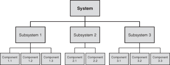
Figure 9.2. Traditional hierarchical block diagram.
The block diagram is seen to be a very abstract model, focusing solely on the units of the system structure and their physical relationships. The simple rectangular blocks are strictly symbolic, with no attempt to depict the physical form of the system elements. However, the diagram does communicate very clearly an important type of relationship among the system elements, as well as identify the system’s organizing principle. More complex interactions across the subsystems and components are left to more detailed diagrams and descriptions. The interactions among blocks may be represented by labeling the connecting lines.
System Context Diagrams.
Another useful model in system design is the context diagram, which represents all external entities that may interact with a system, either directly or indirectly. We have already seen the context diagram in Figure 3.2. Such a diagram pictures the system at the center, with no details of its interior structure, surrounded by all its interacting systems, environments, and activities. The objective of a system context diagram is to focus attention on external factors and events that should be considered in developing a complete set of system requirements and constraints. In so doing, it is necessary to visualize not only the operational environment but also the stages leading up to operations, such as installation, integration, and operational evaluation.
Figure 9.3 shows a context diagram for the case of a passenger airliner. The model represents the external relationships between the airliner and various external entities. The system context diagram is a useful starting point for describing and defining the system’s mission and operational environment, showing the interaction of a system with all external entities that may be relevant to its operation. It also provides a basis for formulating system operational scenarios that represent the different conditions under which it must be designed to operate. In commercial systems, the “enterprise diagram” also shows all the system’s external inputs and outputs but also usually includes a representation of the related external entities.

Figure 9.3. Context diagram of a passenger aircraft.
Functional Flow Block Diagrams (FFBDs).
The models discussed previously deal primarily with static relationships within the system’s physical structure. The more significant characteristics of systems and their components are related to how they behave in response to changes in the environment. Such behavior results from the functions that a system performs in response to certain environmental inputs and constraints. Hence, to model system behavior, it is necessary to model its principal functions, how they are derived, and how they are related to one another. The most common form of functional model is called the FFBD.
An example of an FFBD is shown in Figure 9.4. The figure shows the functional flow through an air defense system at the top-level functions of detect, control, and engage, and at the second-level functions that make up each of the above. Note the numbering system of the functional blocks that ties them together. Note also that the names in the blocks represent functions, not physical entities, and thus, all begin with a verb instead of a noun. The arrowheads on the lines between blocks in an FFBD indicate the flow of control and, in this case, also the flow of information. Keep in mind that flow of control does not necessarily equate with flow of information in all cases. The identity of the functions flowing between the blocks may be denoted on the FFBD as an optional feature but is not expected to be complete as it would be in a software DFD.

Figure 9.4. Air defense functional flow block diagram.
In the above example, the physical implementation of the functional blocks is not represented and may be subject to considerable variation. From the nature of the functions, however, it may be inferred that a radar installation may be involved in the detection function, along with very considerable software; that the control function is mostly software with operator displays; and that the engage function is largely hardware, such as guns, missiles, or aircraft.
A valuable application of functional flow diagrams was developed by the then Radio Corporation of America, Moorestown Division. Named the functional flow diagrams and descriptions (F2D2), the method is used to diagram several functional levels of the system hierarchy, from the system level down to subcomponents. The diagrams use distinctive symbols to identify hardware, software, and people functions, and show the data that flow between system elements. An important use of F2D2 diagrams is in a “war room” or storyboard arrangement, where diagrams for all subsystems are arranged on the walls of a conference room and linked to create a diagram of the entire system. Such a display makes an excellent communication and management tool during the system design process.
DFDs.
DFDs are used in the software structural analysis methodology to model the interactions among the functional elements of a computer program. DFDs have also been used to represent the data flow among physical entities in systems consisting of both hardware and software components. In either case, the labels represent data flow and are labeled with a description of the data traversing the interface.
Integrated Definition Language 0 (IDEF0) Diagrams.
IDEF0 is a standard representation of system activity models, similar to software DFDs, and was described in Chapter 8. Figure 8.3 depicts the rules for depicting an activity. IDEF0 is widely used in the modeling of complex information systems. As in FFBD and F2D2 diagrams, the functional blocks are rectangular and the sides of the activity boxes have a unique function. Processing inputs always enter from the left, controls from the top, and mechanisms or resources from the bottom; outputs exit on the right. The name of each block starts with a vowel and carries a label identifying its hierarchical location.
Functional Flow Process Diagrams (FFPD).
The functional flow diagrams described earlier model the functional behavior of a system or a system product. Such diagrams are equally useful in modeling processes, including those involved in systems engineering. Examples of FFPDs are found in every chapter. The system life cycle model is a prime example of a process FFPD. In Chapter 4, Figures 4.1, 4.3, and 4.4 define the flow of system development through the defined stages and phases of the system life cycle. In Chapters 5–8, the first figures show the functional inputs and outputs between the corresponding life cycle phase and those immediately adjoining.
The systems engineering method is modeled in Chapter 4, Figure 4.10, and in greater detail in Figure 4.11. The functional blocks in this case are the principal processes that constitute the systems engineering method. Inside each block is a functional flow diagram that represents the functions performed by the block. The inputs coming from outside the blocks represent the external factors that contribute to the respective processes. Chapters 5–8 contain similar functional flow diagrams to illustrate the processes that take place during each phase of system development.
FFPDs are especially useful as training aids for production workers by resolving complex processes into their elementary components in terms readily understandable by the trainees. All process diagrams have a common basic structure, which consists of three elements: input → processing → output.
Trigonal System Models.
In attempting to understand the functioning of complex systems, it is useful to resolve them into subsystems and components that individually are more simple to understand. A general method that works well in most cases is to resolve the system and each of its subsystems into three basic components:
- 1. sensing or inputting signals, data, or other media that the system element operates on;
- 2. processing the inputs to deduce an appropriate reaction to the inputs; and
- 3. acting on the basis of the instructions from the processing element to implement the system element’s response to the input.
In an example of a system simulation described in the previous subsection, an air defense system was shown to be composed of three functions, namely, detect, control, and engage (see Fig. 9.4). The detect function is seen to correspond to the input portion, control (or analyze and control response) to the processing portion, and engage to the response action portion.
The input–processing–output segmentation can then be applied to each of the subsystems themselves. Thus, in the air defense system example, the detect function can be further resolved into the radar, which senses the reflection from the enemy airplane or missile, the radar signal processor, which resolves the target reflection from interfering clutter and jamming, and the automatic detection and track software, which correlates the signal with previous scans to form a track and calculate its coordinates and velocity vector for transmission to the control subsystem. The other two subsystems may be similarly resolved.
In many systems, there is more than a single input. For example, the automobile is powered by fuel but is steered by the driver. The input–processing–output analysis will produce two or more functional flows: tracing the fuel input will involve the fuel tank and fuel pump, which deliver the fuel, the engine, which converts (processes) the fuel into torque, and the wheels, which produce traction on the road surface to propel the car. A second set of components are associated with steering the car, in which the sensing and decision is accomplished by the driver, with the automobile executing the actual turn in response to steering wheel rotation.
Modeling Languages.
The schematic models described above together were developed relatively independently. Thus, although they have been in use for several decades, they are used according to the experience of the engineer. However, these models do have certain attributes in common. They are, by and large, activity focused. They communicate functionality of systems, whether that is of the form of activities, control, or data. Even block diagrams representing physical entities include interfaces among the entities showing flow of materials, energy, or data. Because of their age (basic block diagrams have been around for over 100 years), we tend to categorize these models as “functional” or “traditional.”
When software engineering emerged as a significant discipline within system development, a new perspective was presented to the engineering community: object-oriented analysis (OOA). Rather than activity based, OOA presented concepts and models that were object based, where object is defined in very broad terms. Theoretically, anything can be an object. As described in Chapter 8, Unified Modeling Language (UML) is now a widely used modeling language for support of systems engineering and architecting.
Mathematical Models
Mathematical models are used to express system functionality and dependencies in the language of mathematics. They are most useful where system elements can be isolated for purposes of analysis and where their primary behavior can be represented by well-understood mathematical constructs. If the process being modeled contains random variables, simulation is likely to be a preferable approach. An important advantage of mathematical models is that they are widely understood. Their results have inherent credibility, provided that the approximations made can be shown to be of secondary importance. Mathematical models include a variety of forms that represent deterministic (not random) functions or processes. Equations, graphs, and spreadsheets, when applied to a specific system element or process, are common examples.
Approximate Calculations.
Chapter 1 contains a section entitled The Power of Systems Engineering, which cites the critical importance of the use of approximate (“back of the envelope”) calculations to the practice of systems engineering. The ability to perform “sanity checks” on the results of complex calculations or experiments is of inestimable value in avoiding costly mistakes in system development.
Approximate calculations represent the use of mathematical models, which are abstract representations of selected functional characteristics of the system element being studied. Such models capture the dominant variables that determine the main features of the outcome, omitting higher-order effects that would unduly complicate the mathematics. Thus, they facilitate the understanding of the primary functionality of the system element.
As with any model, the results of approximate calculations must be interpreted with full knowledge of their limitations due to the omission of variables that may be significant. If the sanity check deviates significantly from the result being checked, the approximations and other assumptions should be examined before questioning the original result.
In developing the skill to use approximate calculations, the systems engineer must make the judgment as to how far to go into the technical fundamentals in each specific case. One alternative is to be satisfied with an interrogation of the designers who made the original analysis. Another is to ask an expert in the discipline to make an independent check. A third is to apply the systems engineer’s own knowledge, to augment it by reference to a handbook or text, and to carry out the approximate calculation personally.
The appropriate choice among these alternatives is, of course, situation dependent. However, it is advisable that in selected critical technical areas, the systems engineer becomes sufficiently familiar with the fundamentals to feel comfortable in making independent judgments. Developing such skills is part of the systems engineer’s special role of integrating multidisciplinary efforts, assessing system risks, and deciding the areas that require analysis, development, or experimentation.
Elementary Relationships.
In every field of engineering and physics, there are some elementary relationships with which the systems engineer should be aware, or familiar. Newton’s laws are applicable in all vehicular systems. In the case of structural elements under stress, it is often useful to refer to relationships involving strength and elastic properties of beams, cylinders, and other simple structures. With electronic components, the systems engineer should be familiar with the elementary properties of electronic circuits. There are “rules of thumb” in most technical fields, which are usually based on elementary mathematical relationships.
Statistical Distributions.
Every engineer is familiar with the Gaussian (normal) distribution function characteristic of random noise and other simple natural effects. Some other distribution functions that are of interest include the Rayleigh distribution, which is valuable in analyzing signals returned from radar clutter, the Poisson distribution, the exponential distribution, and the binomial distribution; all of these obey simple mathematical equations.
Graphs.
Models representing empirical relationships that do not correspond to explicit mathematical equations are usually depicted by graphs. Figure 2.1a in Chapter 2 is a graph illustrating the typical relationship between performance and the cost to develop it. Such models are mainly used to communicate qualitative concepts, although test data plotted in the form of a graph can show a quantitative relationship. Bar charts, such as one showing the variations in production by month, or the cost of alternative products, are also models that serve to communicate relationships in a more effective manner than by a list of numbers.
Physical Models
Physical models directly reflect some or most of the physical characteristics of an actual system or system element under study. In that sense, they are the least abstract and therefore the most easily understood type of modeling. Physical models, however, are by definition simplifications of the modeled articles. They may embody only a part of the total product; they may be scaled-down versions or developmental prototypes. Such models have multiple uses throughout the development cycle, as illustrated by the examples described next.
Scale Models.
These are (usually) small-scale versions of a building, vehicle, or other system, often used to represent the external appearance of a product. An example of the engineering use of scale models is the testing of a model of an air vehicle in a wind tunnel or of a submersible in a water tunnel or tow tank.
Mock-Ups.
Full-scale versions of vehicles, parts of a building, or other structures are used in later stages of development of systems containing accommodation for operators and other personnel. These provide realistic representations of human–system interfaces to validate or possibly to modify their design prior to a detailed design of the interfaces.
Prototypes.
Previous chapters have discussed the construction and testing of development, engineering, and product prototypes, as appropriate to the system in hand. These also represent physical models of the system, although they possess most of the properties of the operational system. However, strictly speaking, they are still models.
Computer-based tools are being increasingly used in place of physical models such as mock-ups and even prototypes. Such tools can detect physical interferences and permit many engineering tasks formerly done with physical models to be accomplished with computer models.
9.4 SIMULATION
System simulation is a general type of modeling that deals with the dynamic behavior of a system or its components. It uses a numerical computation technique for conducting experiments with a software model of a physical system, function, or process. Because simulation can embody the physical features of the system, it is inherently less abstract than many forms of modeling discussed in the previous section. On the other hand, the development of a simulation can be a task of considerable magnitude.
In the development of a new complex system, simulations are used at nearly every step of the way. In the early phases, the characteristics of the system have not yet been determined and can only be explored by modeling and simulation. In the later phases, estimates of their dynamic behavior can usually be obtained earlier and more economically by using simulations than by conducting tests with hardware and prototypes. Even when engineering prototypes are available, field tests can be augmented by using simulations to explore system behavior under a greater variety of conditions. Simulations are also used extensively to generate synthetic system environmental inputs for test purposes. Thus, in every phase of system development, simulations must be considered as potential development tools.
There are many different types of simulations and one must differentiate static from dynamic simulations, deterministic from stochastic (containing random variables), and discrete from continuous. For the purposes of relating simulations to their application to systems engineering, this section groups simulations into four categories: operational, physical, environmental, and virtual reality simulation. All of these are either wholly or partly software based because of the versatility of software to perform an almost infinite variety of functions.
Computer-based tools also perform simulations at a component or subcomponent level, which will be referred to as engineering simulation.
Operational Simulation
In system development, operational simulations are primarily used in the conceptual development stage to help define operational and performance requirements, explore alternative system concepts, and help select a preferred concept. They are dynamic, stochastic, and discrete event simulations. This category includes simulations of operational systems capable of exploring a wide range of scenarios, as well as system variants.
Games
The domain of analyzing operational mission areas is known as operations analysis. This field seeks to study operational situations characteristic of a type of commerce, warfare, or other broad activity and to develop strategies that are most suitable to achieving successful results. An important tool of operations analysis is the use of games to evaluate experimentally the utility of different operational approaches. The military is one of the organizations that relies on games, called war games, to explore operational considerations.
Computer-aided games are examples of operational simulations involving people who control a simulated system (blue team) in its engagement with the simulated adversary (red team), with referees observing both sides of the action and evaluating the results (white team). In business games, the two sides represent competitors. In other games, the two teams can represent adversaries.
The behavior of the system(s) involved in a game is usually based on that of existing operational systems, with such extensions as may be expected to be possible in the next generation of the system. These may be implemented by variable parameters to explore the effect of different system features on their operational capabilities.
Gaming has several benefits. First, it enables the participants to gain a clearer understanding of the operational factors involved in various missions, as well as of their interaction with different features of the system, which translates into experience in operational decision making. Second, by varying key system features, the participants can explore system improvements that may be expected to enhance their effectiveness. Third, through variation in operational strategy, it may be possible to develop improved operational processes, procedures, and methods. Fourth, analysis of the game results may provide a basis for developing a more clearly stated and prioritized set of operational requirements for an improved system than could be derived otherwise.
Commercial games are utilized by large corporations to identify and assess business strategies over a single and multiple business cycles within a set of plausible economic scenarios. Although these games do not typically predict technological breakthroughs, they can identify “breakthrough” technologies that could lead to paradigm shifts in an industry.
Military organizations conduct a variety of games for multiple purposes such as assessing new systems within a combat situation, analyzing a new concept for transporting people and material, or evaluating a new technology to detect stealthy targets. The games are facilitated by large screen displays and a bank of computers. The geographic displays are realistic, derived from detailed maps of the globe available on the Internet and from military sources. A complex game may last from a day to several weeks. The experience is highly enlightening to all participants. Short of actual operational experience, such games are the best means for acquiring an appreciation of the operational environment and mission needs, which are important ingredients in systems engineering.
Lastly, government organizations and alliances conduct geopolitical games to assess international engagement strategies. These types of games tend to be complex as the dimensions of interactions can become quite large. For example, understanding national reactions to a country’s policy actions involves diplomatic, intelligence, military, and economic (DIME) ramifications. Also, because interactions are complex, standard simulation types may not be adequate to capture the realm of actions that a nation might take. Therefore, sophisticated simulations are developed specifically to model various components of a national entity. These components are known as agents.
System Effectiveness Simulation
During the concept exploration and concept definition phases of system development, the effort is focused on the comparative evaluation of different system capabilities and architectures. The objective is first to define the appropriate system performance requirements and then to select the preferred system concept to serve as the basis for development. A principal vehicle for making these decisions is the use of computer system effectiveness simulations, especially in the critical activity of selecting a preferred system concept during concept definition. At this early point in the system life cycle, there is neither time nor resources to build and test all elements of the system. Further, a well-designed simulation can be used to support the claimed superiority of the system concept recommended to the customer. Modern computer display techniques can present system operation in realistic scenarios.
The design of a simulation of a complex system that is capable of providing a basis for comparing the effectiveness of candidate concepts is a prime systems engineering task. The simulation itself is likely to be complex in order to reflect all the critical performance factors. The evaluation of system performance also requires the design and construction of a simulation of the operational environment that realistically challenges the operational system’s capabilities. Both need to be variable to explore different operational scenarios, as well as different system features.
A functional block diagram of a typical system effectiveness simulation is illustrated in Figure 9.5. The subject of the simulation is an air defense system, which is represented by the large rectangle in the center containing the principal subsystems detect, control, and engage. At the left is the simulation of the enemy force, which contains a scenario generator and an attack generator. At the right is the analysis subsystem, which assesses the results of the engagement against an expected outcome or against results from other engagements. The operator interface, shown at the bottom, is equipped to modify the attacking numbers and tactics and also to modify the performance of these system elements to determine the effects on system effectiveness.

Figure 9.5. System effectiveness simulation.
The size and direction of system effectiveness variations resulting from changes in the system model should be subjected to sanity checks before acceptance. Such checks involve greatly simplified calculations of the system performance and are best carried out by analysts not directly responsible for either the design or the simulation.
Mission Simulation
The objective of the simulations referred to as mission simulations is focused on the development of the operational modes of systems rather than on the development of the systems themselves. Examples of such simulations include the conduct of air traffic control, the optimum trajectories of space missions, automobile traffic management, and other complex operations.
For example, space missions to explore planets, asteroids, and comets are preceded by exhaustive simulations of the launch, orbital mechanics, terminal maneuvers, instrument operations, and other vital functions that must be designed into the spacecraft and mission control procedures. Before design begins, an analytical foundation using simulation techniques is developed.
Such simulations model the vehicles and their static and dynamic characteristics, the information available from various sensors, and significant features of the environment and, if appropriate, present these items to the system operator’s situation displays mimicking what they would see in real operations. The simulations can be varied to present a variety of possible scenarios, covering the range of expected operational situations. Operators may conduct “what if” experiments to determine the best solution, such as a set of rules, a safe route, an optimum strategy, or whatever the operational requirements call for.
Physical Simulation
Physical simulations model the physical behavior of system elements. They are primarily used in system development during the engineering development stage to support systems engineering design. They permit the conduct of simulated experiments that can answer many questions regarding the fabrication and testing of critical components. They are dynamic, deterministic, and continuous.
The design of all high-performance vehicles—land, sea, air, or space—depends critically on the use of physical simulations. Simulations enable the analyst and designer to represent the equations of motion of the vehicle, the action of external forces, such as lift and drag, and the action of controls, whether manual or automated. As many experiments as may be necessary to study the effects of varying conditions or design parameters may be conducted. Without such tools, the development of modern aircraft and spacecraft would not have been practicable. Physical simulations do not eliminate the need for exhaustive testing, but they are capable of studying a great variety of situations and of eliminating all but a few alternative designs. The savings in development time can be enormous.
Examples: Aircraft, Automobiles, and Space Vehicles.
Few technical problems are as complicated as the design of high-speed aircraft. The aerodynamic forces are quite nonlinear and change drastically in going between subsonic and supersonic regimes. The stresses on airplane structures can be extremely high, resulting in flexure of wings and control surfaces. There are flow interference effects between the wings and tail structure that depend sharply on altitude, speed, and flight attitude. Simulation permits all of these forces and effects to be realistically represented in six-degree-of-freedom models (three position and three rotation coordinates).
The basic motions of an automobile are, of course, far simpler than those of an aircraft. However, modern automobiles possess features that call on very sophisticated dynamic analysis. The control dynamics of antilock brakes are complex and critical, as are those of traction control devices. The action of airbag deployment devices is even more critical and sensitive. Being intimately associated with passenger safety, these devices must be reliable under all expected conditions. Here again, simulation is an essential tool.
Without modern simulation, there would be no space program as we know it. The task of building a spacecraft and booster assembly that can execute several burns to put the spacecraft into orbit, that can survive launch, deploy solar panels, and antennae, control its attitude for reasons of illumination, observation, or communication, and perform a series of experiments in space would simply be impossible without a variety of simulations. The international space station program achieved remarkable sustainability as each mission was simulated and rehearsed to near perfection.
Hardware-in-the-Loop Simulation
This is a form of physical simulation in which actual system hardware is coupled with a computer-driven simulation. An example of such a simulation is a missile homing guidance facility. For realistic experiments of homing dynamics, such a facility is equipped with microwave absorbing materials, movable radiation sources, and actual seeker hardware. This constitutes a dynamic “hardware-in-the-loop” simulation, which realistically represents a complex environment.
Another example of a hardware-in-the-loop simulation is a computer-driven motion table used in the development testing of inertial components and platforms. The table is caused to subject the components to movement and vibration representing the motion of its intended platform, and is instrumented to measure the accuracy of the resulting instrument output. Figure 9.6 shows a developmental inertial platform mounted on a motion table, with a motor drive controlled by an operator and the feedback from the platform. A motion analyzer compares the table motion with the inertial platform outputs.

Figure 9.6. Hardware-in-the-loop simulation.
Engineering Simulation
At the component and subcomponent level, there are engineering tools that are extensions of mathematical models, described in the previous section. These are primarily used by design specialists, but their capabilities and limitations need to be understood by systems engineers in order to understand their proper applications.
Electronic circuit design is no longer done by cut-and-try methods using breadboards. Simulators can be used to design the required functionality, test it, and modify it until the desired performance is obtained. Tools exist that can automatically document and produce a hardware version of the circuit.
Similarly, the structural analysis of complex structures such as buildings and bridges can be done with the aid of simulation tools. This type of simulation can accommodate the great number of complicated interactions among the mechanical elements that make up the structure, which are impractical to accomplish by analysis and testing.
Development of the Boeing 777 Aircraft
As noted previously, virtually all of the structural design of the Boeing 777 was done using computer-based modeling and simulation. One of the aircraft’s chief reasons for success was the great accuracy of interface data that allowed the various portions of the aircraft to be designed and built separately and then to be easily integrated. This technology set the stage for the Boeing 797, the Dreamliner.
The above techniques have literally revolutionized many aspects of hardware design, development, testing, and manufacture. It is essential for systems engineers working in these areas to obtain a firsthand appreciation of the application and capability of engineering simulation to be able to lead effectively the engineering effort.
Environmental Simulation
Environmental simulations are primarily used in system development during engineering test and evaluation. They are a form of physical simulation in which the simulation is not of the system but of elements of the system’s environment. The majority of such simulations are dynamic, deterministic, and discrete events.
This category is intended to include simulation of (usually hazardous) operating environments that are difficult or unduly expensive to provide for validating the design of systems or system elements, or that are needed to support system operation. Some examples follow.
Mechanical Stress Testing.
System or system elements that are designed to survive harsh environments during their operating life, such as missiles, aircraft systems, spacecraft, and so on, need to be subjected to stresses simulating such conditions. This is customarily done with mechanical shake tables, vibrators, and shock testing.
Crash Testing.
To meet safety standards, automobile manufacturers subject their products to crash tests, where the automobile body is sacrificed to obtain data on the extent to which its structural features lessen the injury suffered by the occupant. This is done by use of simulated human occupants, equipped with extensive instrumentation that measures the severity of the blow resulting from the impact. The entire test and test analysis are usually computer driven.
Wind Tunnel Testing.
In the development of air vehicles, an indispensable tool is an aerodynamic wind tunnel. Even though modern computer programs can model the forces of fluid flow on flying bodies, the complexity of the behavior, especially near the velocity of sound, and interactions between different body surfaces often require extensive testing in facilities that produce controlled airflow conditions impinging on models of aerodynamic bodies or components. In such facilities, the aerodynamic model is mounted on a fixture that measures forces along all components and is computer controlled to vary the model angle of attack, control surface deflection, and other parameters, and to record all data for subsequent analysis.
As noted in the discussion of scale models, analogous simulations are used in the development of the hulls and steering controls of surface vessels and submersibles, using water tunnels and tow tanks.
Virtual Reality Simulation
The power of modern computers has made it practical to generate a three-dimensional visual environment of a viewer that can respond to the observer’s actual or simulated position and viewing direction in real time. This is accomplished by having all the coordinates of the environment in the database, recomputing the way it would appear to the viewer from his or her instantaneous position and angle of sight, and projecting it on a screen or other display device usually mounted in the viewer’s headset. Some examples of the applications of virtual reality simulations are briefly described next.
Spatial Simulations.
A spatial virtual reality simulation is often useful when it is important to visualize the interior of enclosed spaces and the connecting exits and entries of those spaces. Computer programs exist that permit the rapid design of these spaces and the interior furnishings. A virtual reality feature makes it possible for an observer to “walk” through the spaces in any direction. This type of model can be useful for the preliminary designs of houses, buildings, control centers, storage spaces, parts of ships, and even factory layouts. An auxiliary feature of this type of computer model is the ability to print out depictions in either two- or three-dimensional forms, including labels and dimensions.
Spatial virtual simulations require the input to the computer of a detailed three-dimensional description of the space and its contents. Also, the viewing position is input into the simulation either from sensors in the observer’s headset or directed with a joystick, mouse, or other input device. The virtual image is computed in real time and projected either to the observer’s headset or on a display screen. Figure 9.7 illustrates the relationship between the coordinates of two sides of a room with a bookcase on one wall, a window on the other, and a chair in the corner, and a computer-generated image of how an observer facing the corner would see it.

Figure 9.7. Virtual reality simulation.
Video Games.
Commercial video games present the player with a dynamic scenario with moving figures and scenery that responds to the player’s commands. In many games, the display is fashioned in such a way that the player has the feeling of being inside the scene of the action rather than of being a spectator.
Battlefield Simulation.
A soldier on a battlefield usually has an extremely restricted vision of the surroundings, enemy positions, other forces, and so on. Military departments are actively seeking ways to extend the soldier’s view and knowledge by integrating the local picture with situation information received from other sources through communication links. Virtual reality techniques are expected to be one of the key methods of achieving these objectives of situational awareness.
Development of System Simulations
As may be inferred from this section, the several major simulations that must be constructed to support the development of a complex system are complex in their own right. System effectiveness simulations have to not only simulate the system functionality but also to simulate realistically the system environment. Furthermore, they have to be designed so that their critical components may be varied to explore the performance of alternative configurations.
In Chapter 5, modeling and simulation were stated to be an element of the systems engineering management plan. In major new programs, the use of various simulations may well account for a substantial portion of the total cost of the system development. Further, the decisions on the proper balance between simulation fidelity and complexity require a thorough understanding of the critical issues in system design, technical and program risks, and the necessary timing for key decisions. In the absence of careful analysis and planning, the fidelity of simulations is likely to be overspecified, in an effort to prevent omissions of key parameters. The result of overambitious fidelity is the extension of project schedules and exceedance of cost goals. For these reasons, the planning and management of the system simulation effort should be an integral part of systems engineering and should be reflected in management planning.
Often the most effective way to keep a large simulation software development within bounds is to use iterative prototyping, as described in Chapter 11. In this instance, the simulated system architecture is organized as a central structure that performs the basic functions, which is coupled to a set of separable software modules representing the principal system operational modes. This permits the simulation to be brought to limited operation quickly, with the secondary functions added, as time and effort are available.
Simulation Verification and Validation
Because simulations serve an essential and critical function in the decision making during system development, it is necessary that their results represent valid conclusions regarding the predicted behavior of the system and its key elements. To meet this criterion, it must be determined that they accurately represent the developer’s conceptual description and specification (verification) and are accurate representations of the real world, to the extent required for their intended use (validation).
The verification and validation of key simulations must, therefore, be an integral part of the total system development effort, again under the direction of systems engineering. In the case of new system effectiveness simulations, which are usually complex, it is advisable to examine their results for an existing (predecessor) system whose effectiveness has been previously analyzed. Another useful comparison is with the operation of an older version of the simulation, if one exists.
Every simulation that significantly contributes to a system development should also be documented to the extent necessary to describe its objectives, performance specifications, architecture, concept of operation, and user modes. A maintenance manual and user guide should also be provided.
The above actions are sometimes neglected to meet schedules and in competition with other activities. However, while simulations are not usually project deliverables, they should be treated with equal management attention because of their critical role in the success of the development.
Even though a simulation has been verified and validated, it is important to remember that it is necessarily only a model, that is, a simplification and approximation to reality. Thus, there is no such thing as an absolutely validated simulation. In particular, it should only be used for the prescribed application for which it has been tested. It is the responsibility of systems engineering to circumscribe the range of valid applicability of a given simulation and to avoid unwarranted reliance on the accuracy of its results.
Despite these cautions, simulations are absolutely indispensable tools in the development of complex systems.
9.5 TRADE-OFF ANALYSIS
Performing a trade-off is what we do whenever we make a decision, large or small. When we speak, we subconsciously select words that fit together to express what we mean, instinctively rejecting alternative combinations of words that might have served the purpose, but not as well. At a more purposeful level, we use trade-offs to decide what to wear to a picnic or what flight to take on a business trip. Thus, all decision processes involve choices among alternative courses of action. We make a decision by comparing the alternatives against one another and by choosing the one that provides the most desirable outcome.
In the process of developing a system, hundreds of important systems engineering decisions have to be made, many of them with serious impacts on the potential success of the development. Those cases in which decisions have to be approved by management or by the customer must be formally presented, supported by evidence attesting to the thoroughness and objectivity of the recommended course of action. In other cases, the decision only has to be convincing to the systems engineering team. Thus, the trade-off process needs to be tailored to its ultimate use. To differentiate a formal trade-off study intended to result in a recommendation to higher management from an informal decision aid, the former will be referred to as a “trade-off analysis” or a “trade study,” while the latter will be referred to as simply a “trade-off.” The general principles are similar in both cases, but the implementation is likely to be considerably different, especially with regard to documentation.
Basic Trade-Off Principles
The steps in a trade-off process can be compared to those characterizing the systems engineering methodology, as used in the systems concept definition phase for selecting the preferred system concept to meet an operational objective. The basic steps in the trade-off process at any level of formality are the following (corresponding steps in the systems engineering methodology are shown in parentheses).
Defining the Objective (Requirements Analysis).
The trade-off process must start by defining the objectives for the trade study itself. This is carried out by identifying the requirements that the solution (i.e., the result of the decision) must fulfill. The requirements are best expressed in terms of measures of effectiveness (MOE), as quantitatively as practicable, to characterize the merits of a candidate solution.
Identification of Alternatives (Concept Exploration).
To provide a set of alternative candidates, an effort must be made to identify as many potential courses of action as will include all promising candidate alternatives. Any that fail to comply with an essential requirement should be rejected.
Comparing the Alternatives (Concept Definition).
To determine the relative merits of the alternatives, the candidate solutions should be compared with one another with respect to each of their MOEs. The relative order of merit is judged by the cumulative rating of all the MOEs, including a satisfactory balance among the different MOEs.
Sensitivity Analysis (Concept Validation).
The results of the process should be validated by examining their sensitivity to the assumptions. MOE prioritization and candidate ratings are varied within limits reflecting the accuracy of the data. Candidates rated low in only one or two MOEs should be reexamined to determine whether this result could be changed by a relatively straightforward modification. Unless a single candidate is clearly superior, and the result is stable to such variations, further study should be conducted.
Formal Trade-Off Analysis and Trade Studies
As noted above, when trade-offs are conducted to derive and support a recommendation to management, they must be performed and presented in a formal and thoroughly documented manner. As distinguished from informal decision processes, trade-off studies in systems engineering should have the following characteristics:
- 1. They are organized as defined processes. They are carefully planned in advance, and their objective, scope, and method of approach are established before they are begun.
- 2. They consider all key system requirements. System cost, reliability, maintainability, logistics support, growth potential, and so on, should be included. Cost is frequently handled separately from other criteria. The result should demonstrate thoroughness.
- 3. They are exhaustive. Instead of considering only the obvious alternatives in making a systems engineering decision, a search is made to identify all options deserving consideration to ensure that a promising one is not inadvertently overlooked. The result should demonstrate objectivity.
- 4. They are semiquantitative. While many factors in the comparison of alternatives may be only approximately quantifiable, systems engineering trade-offs seek to quantify all possible factors to the extent practicable. In particular, the various MOEs are prioritized relative to one another in order that the weighting of the various factors achieves the best balance from the standpoint of the system objectives. All assumptions must be clearly stated.
- 5. They are thoroughly documented. The results of systems engineering trade-off analyses must be well documented to allow review and to provide an audit trail should an issue need reconsideration. The rationale behind all weighting and scoring should be clearly stated. The results should demonstrate logical reasoning.
A formal trade study leading to an important decision should include the steps described in the following paragraphs. Although presented linearly, many overlap and several can be, and should be, coupled together in an iterative subprocess.
Step 1: Definition of the Objectives.
To introduce the trade study, the objectives must be clearly defined. These should include the principal requirements and should identify the mandatory ones that all candidates must meet. The issues that will be involved in selecting the preferred solution should also be included. The objectives should be commensurate with the phase of system development. The operational context and the relationships to other trade studies should be identified at this time. Trade studies conducted early in the system development cycle are typically conducted at the system level and higher. Detailed component-level trade studies are conducted later, during engineering and implementation phases.
Step 2: Identification of Viable Alternatives.
As stated previously, before embarking on a comparative evaluation, an effort should be made to define several candidates to ensure that a potentially valuable one is not overlooked. A useful strategy for finding candidate alternatives is to consider those that maximize a particularly important characteristic. Such a strategy is illustrated in the section on concept selection in Chapter 8, in which it is suggested to consider candidates based on the following:
- the predecessor system as a baseline,
- technological advances,
- innovative concepts, and
- candidates suggested by interested parties.
In selecting alternatives, no candidate should be included that does not meet the mandatory requirements, unless it can be modified to qualify. However, keep the set of mandatory requirements small. Sometimes, an alternative concept that does not quite meet a mandatory requirement but is superior in other categories, or results in significant cost savings, is rejected because it does not reach a certain threshold. Ensure that all mandatory requirements truly are mandatory—and not simply someone’s guess or wish.
The factors to consider in developing the set of alternatives are the following:
- There is never a single possible solution. Complex problems can be solved in a variety of ways and by a variety of implementations. In our experience, we have never encountered a problem with one and only one solution.
- Finding the optimal solution is rarely worth the effort. In simple terms, systems engineering can be thought of as the art and science of finding the “good enough” solution. Finding the mathematical optimum is expensive and many times near impossible.
- Understand the discriminators among alternatives. Although the selection criteria are not chosen at this step (this is the subject of the next step), the systems engineer should have an understanding of what discriminates alternatives. Some discriminators are obvious and exist regardless of the type of system you are developing: cost, technical risk, reliability, safety, and quality. Even of some of these cannot be quantified, yet a basic notion of how alternatives discriminate within these basic categories will enable the culling of alternatives to a reasonable quantity.
- Remain open to additional solutions surfacing during the trade study. This step is not forgotten once an initial set of alternatives has been identified. Many times, even near the end of the formal trade study, additional options may emerge that hold promise. Typically, a new option arises that combines the best features of two or more original alternatives. Many times, identifying these alternatives is not possible, or at least difficult, early in the process.
Staged Process.
This step tends to occur in discrete stages. Initially, a large number and variety of alternatives should be considered. Brainstorming is one effective method of capturing a variety of alternatives, without evaluating their merits. Challenge participants to think “out of the box” to ensure that no option is overlooked. And while some ridiculous ideas are offered, this tends to stimulate thinking on other, plausible options. In our experience, 40–50 alternatives can be identified initially. This set is not our final set of alternatives, of course. It needs to be reduced.
As long as there are more than three to five potential alternatives, it is suggested that the staged approach be continued, culling the set down to a manageable set. The process of reducing alternatives generally follows a rank-ordering process, rather than quantitative weighing and scoring, to weed out less desirable candidates. Options can be dismissed due to a variety of reasons: cost, technological feasibility, safety, manufacturability, operational risk, and so on. This process may also uncover criteria that are not useful differentiators. Follow-on stages would focus on a few candidates that include likely candidates. These would be subjected to a much more thorough analysis as described below.
Remember to document the choices and reasoning behind the decision. Include the specifications for the alternatives to make the trade-off as quantitative as possible. The result of this multistage process is a reasonable set of alternatives that can be evaluated formally and comprehensively.
Step 3: Definition of Selection Criteria.
The basis of differentiating between alternative solutions is a set of selection criteria to be chosen from and referenced to the requirements that define the solution. Each criterion must be an essential attribute of the product, expressed as a MOE, related to one or more of its requirements. It is desirable that it be quantifiable so that its value for each alternative may be derived objectively. Cost is almost always a key criterion. Reliability and maintainability are also usually important characteristics, but they must be quantified. In the case of large systems, size, weight, and power requirements can be important criteria. In software products, ease of use and supportability are usually important differentiators.
Characteristics that are possessed by all candidates to a comparable degree do not serve to distinguish among them and hence should not be used, because their inclusion only tends to obscure the significant discriminators. Also, two closely interdependent characteristics do not contribute more discrimination than can be obtained by one of them with appropriate weighting. The number of criteria used in a particular formal trade study can vary widely but usually ranges between 6 and 10. Fewer criteria may not appear convincing of a thorough study. More criteria tend to make the process unwieldy without adding value.
Step 4: Assignment of Weighting Factors to Selection Criteria.
In a given set of criteria, not all of them are equally important in determining the overall value of an alternative. Such differences in importance are taken into account by assigning each criterion a “weighting factor” that magnifies the contribution of the most critical criteria, that is, those to which the total value is the most sensitive, in comparison to the less critical. This procedure often turns out to be troublesome to carry out because many, if not most, of the criteria are incommensurable, such as cost versus risk, or accuracy versus weight. Also, judgments of relative criticality tend to be subjective and often depend on the particular scenario used for the comparison.
Several alternative weighting schemes are available. All of them should engage domain experts to help with the decisions. Perhaps the simplest is to assign weights from 1 to n (with n having the greatest contribution). Although subjective, the criteria are measured relative to each other (as opposed to an absolute measure). A disadvantage with using the typical 1 to n scheme is that people tend to group around the median, in this case, (1 + n)/2. For example, using a 1–5 scale may really be using a 1–3 scale since many will simply not use 1 and 5 often. Other times, people tend to rate all criteria high, either a 4 or 5—resulting in the equivalent of using 1–2.
Adding some objectivity requires a trade-off decision in and of itself when assigning weights. For instance, we could still use the 1–5 scale, but use a maximum number of weighting points; that is, the sum of all of the weights must not exceed a maximum value. A good starting maximum sum might be to take the sum of all average weights,
where
| MaxSum | is the total number of weighting points to be allocated; |
| MaxWeight | is the greatest weight allowed; |
| MinWeight | is the least weight allowed; and |
| n | is the number of criteria. |
Thus, this scheme holds the average weight as a constant. If the engineer (or stakeholders, depending on who is weighting the criteria) wants to weight a criterion higher, then she must reduce the weight of another criterion. Keep in mind, however, with any subjective weighting scheme (any scheme that uses “1 to n”), you are making assumptions about the relative importance. A “5” is five times as relevant as a “1.” These numbers are used in the calculations to compare alternatives. Make sure the scheme is appropriate.
If more mathematical accuracy is desired, the weights could be constrained to sum to 1.0. Thus, each weighting would be a number between 0 and 1.0. This scheme has some mathematical advantages that will be described later in this chapter. One logical advantage is that weightings are not constrained to integers. If one alternative is 50% more important than another, this scheme can represent that relationship; integers cannot. When using spreadsheets for the calculations, be sure not to allow too many significant figures! The credibility of the engineering judgment would fall quickly.
To summarize, deciding on a weighting scheme is important. Careful thinking about the types of relative importance of alternatives is required. Otherwise, the engineer can inadvertently bias the results without knowing.
Step 5: Assignment of Value Ratings for Alternatives.
This step can be confusing to many people. You may ask, why can we not simply measure the criteria values for each alternative at this point and use those values in our comparison? Of course, we could, but it becomes hard to compare the alternatives without integrating the criteria in some manner. Each criterion may use different units; so how does the systems engineer integrate multiple criteria together to gain an understanding of an overall value assessment for each alternative? We cannot combine measures of area (square foot) with velocity (foot per second), for example. And what if a criterion is impossible to measure? Does that mean subjective criteria are simply not used? In fact, subjective criteria are used in system development frequently (though usually in combination with objective criteria). Thus, we need a method to combine criterion together without trying to integrate units that are different. Basically, we need an additional step beyond measuring criterion values for each alternative. We need to assign an effectiveness value.
There are several methods of assigning a value for each criterion to each alternative. Each has its own set of advantages and attributes. And the method ultimately used may not be a choice for the systems engineer, depending on what data can be collected. Three basic options are available: (1) the subjective value method, (2) the step function method, and (3) the utility function method.
The first method relies on the systems engineer’s subjective assessment of the alternative relative to each criterion. The latter two methods use actual measurements and translate the measurement to a value. For example, if volume is a criterion with cubic feet as the unit, then each alternative would be measured directly—what is the volume that each alternative fills, in cubic feet? Combinations of the three methods are also frequently used.
Subjective Value Method.
When this method is chosen, the procedure begins with a judgment of the relative utility of each criterion on a scale analogous to student grading, say 1–5. Thus, 1 = poor, 2 = fair, 3 = satisfactory, 4 = good, and 5 = superior. (A candidate that fails a criterion may be given a zero, or even a negative score if the scores are to be summed, to ensure that the candidate will be rejected despite high scores on other criteria.) This is the effectiveness value for each criterion/alternative pair. The score assigned to the contribution of a given criterion to a specific candidate is the product of the weight assigned to the criterion and the assigned effectiveness value of the candidate in meeting the criterion.
Table 9.3 depicts a generic example that could be constructed for each alternative, for four selection criteria (they are not described, just numbered one through four).
TABLE 9.3. Weighted Sum Integration of Selection Criteria

In this method, the value vi would be an integer between 1 and 5 (using our subjective effectiveness rating above), and would be assigned by the systems engineer.
Actual Measurement Method.
If a more objective effectiveness rating is desired (more than “poor/fair/satisfactory/good/superior”), and alternatives could be measured for each criterion, then a simple mathematical step function could be constructed that translates an actual measurement into an effectiveness value. The systems engineer still needs to define this function and what value will be assigned to what range of measurements. Using our example of volume as a criterion, we could define a step function that assigns an effectiveness value to certain levels of volume. Assuming lesser volume is better effectiveness,
| Volume (ft3) | Value |
| 0–2.0 | 5 |
| 2.01–3.0 | 4 |
| 3.01–4.0 | 3 |
| 4.01–5.0 | 2 |
| >5.0 | 1 |
If an alternative fills 3.47 ft3 of volume, it would be given an effectiveness value of 3. Keep this concept in mind as we will use something similar with our next method.
Table 9.4 illustrates this method. In this case, the alternative is actually measured for each criterion; the result is mi. The step function is then used to translate the measurement to an effectiveness value, vi. The final score for that criterion is the product of the measurement and value, mivi. Once the measurements are converted to values, the actual measurements, mi, are no longer used.
TABLE 9.4. Weighted Sum of Actual Measurement

Utility Function Method.
A refinement of the second approach is to develop a utility function for each criterion, which relates its measurable performance to a number between zero and one. Each criterion is measured, just as in the second method. But instead of allocating subjective values, a utility function is used to map each measurement to a value between zero and one.
Advantages to this method over the second are mathematical. As in using a utility function for weights (i.e., summing the weights to one), using utility functions places all criteria on an equal basis—the effectiveness of each criterion is constrained to a number between zero and one. Furthermore, if utility functions are used, mathematical properties of utility functions can be utilized. These are described in the next section.
Figure 9.8 illustrates some examples of utility functions. A utility function can be either continuous or discrete, linear or nonlinear.

Figure 9.8. Candidate utility functions.
If utility functions are used, calculating a total score for each criterion is similar to the second method. The score is simply the product of the weight and the utility. Table 9.5 depicts these relationships.
TABLE 9.5. Weighted Sum of Utility Scores

Step 6: Calculating Comparative Scores.
The conventional method for combining the scores for the several alternatives is to calculate the sum of the weighted scores for each criterion to produce a total score. The candidate with the greatest summed value is judged to be the best candidate given the selection criteria and weightings, provided the score of the next highest alternative is statistically lower:
This process is simple to implement, but lumping together the scores of the individual criteria tends to obscure factors that may be more important than initially supposed. For example, a candidate may receive a very low score on an essential MOE and high scores on several others. This lack of balance should not be obscured. It is strongly recommended that in addition to presenting the total scores, a graph of the criteria profile for each candidate be also included. Figure 9.9 presents a notional example of a criteria profile for three alternatives.

Figure 9.9. Criteria profile.
Deciding which alternative among the three is best is difficult since Alt-1 scores very low on criterion D but very high on criteria A, B, and C. Is this significant? If only the weighted sums are used, then Alt-1 would be the best candidate (with a sum of 5 + 5 + 4 + 1 = 15). In its purest form, Alt-1 is selected due to its greatest weighted sum, but as always, numbers do not tell the whole story; we need analysis.
Step 7: Analyzing the Results.
Because of the necessary reliance on qualitative judgments and the incommensurable nature of many of the criteria, the results of a trade study should be subjected to critical scrutiny. This process is especially important when the two or three top scores are close together and do not produce a decisive winner.
An essential step in analyzing the results is to examine the individual candidate profiles (scores for each criterion). Candidates that score poorly on one or more criteria may be less desirable than those with satisfactory scores in all categories. Cost is another factor that needs to be considered separately.
The conventional method of summing the individual scores is simple to use but has the unfortunate characteristic of underemphasizing low scores. A technique that does not suffer from this defect is to derive the composite score for a candidate by calculating the product (or geometric mean), rather than the sum, of the individual scores for the several criteria. If a candidate scores a zero on any criterion, the product function will also be zero, rejecting the alternative. An equivalent variant with the same property is to sum the logarithms of the individual scores.
A conventional approach to testing the robustness of trade study results is called “sensitivity analysis.” Sensitivity analysis tests the invariance of the results to small changes in the individual weighting factors and scores. Because of uncertainties in the assignment of weighting and scores, substantial variations (20–30%) should be considered. A preferred approach is to sequentially set each criterion equal to zero and to recalculate the study. When such variations do not change the initial top choice, the procedure builds confidence in the result of the analysis.
An additional sensitivity test is to consider if there are important criteria that have not been included in the evaluation. Examples may be risk, growth potential, availability of support services, maturity of the product or of its supplier, ease of use, and so on. One of the alternatives may be considerably more attractive in regard to several of such additional issues.
Trade-Off Analysis Report.
The results of a formal trade study represent an important milestone in the development of a system or other important operation and will contribute to decisions that will determine the future course. As such, they have to be communicated to all principal participants, who may include customers, managers, technical leaders, and others closely associated with the subject at issue. Such communication takes two forms: presentations and written reports.
Both oral and written reports must contain sufficient material to fully explain the method used and the rationale leading to the conclusions. They should include
- a statement of the issue and requirements on the solution;
- a discussion of assumptions and relationships to other components and subsystems;
- a setting of mission or operational considerations;
- a listing of relevant and critical system or subsystem requirements;
- a description of each alternative selected and the key features that led to its selection;
- an explanation of how the evaluation criteria were selected and the rationale for their prioritization (weighting);
- a rationale for assigning specific scores to each alternative for each criterion;
- a summary of the resulting comparison;
- a description of the sensitivity analysis and its results;
- the final conclusion of the analysis and an evaluation of its validity;
- recommendation for adoption of the study results or further analysis; and
- references to technical, quantitative material.
The presentation has the objective of presenting valuable information to program decision makers in order to make informed decisions. It requires a careful balance between sufficient substance to be clear and too much detail to be confusing. To this end, it should consist mainly of graphical displays, for which the subject is well suited, with a minimum of word charts. On the other hand, it is essential that the rationale for selection weighting and scoring is clear, logical, and persuasive. A copy of the comparison spreadsheet may be useful as a handout.
The purpose of the written trade study report is not only to provide a historical record of the basis for program decisions but also, more importantly, to provide a reference for reviewing the subject if problems arise later in the program. It represents the documented record of the analysis and its results. Its scope affords the opportunity for a detailed account of the steps of the study. For example, it may contain drawings, functional diagrams, performance analysis results, experimental data, and other materials that support the trade-off study.
Trade-Off Analysis Example
An example of a trade-off matrix is illustrated in Table 9.6, for the case of selecting a software code analysis tool. The table compares the ratings of five candidate commercial software tools with respect to six evaluation criteria:
- speed of operation, measured in minutes per run;
- accuracy in terms of errors per 10 runs;
- versatility in terms of number of applications addressed;
- reliability, measured by program crashes per 100 runs;
- user interface, in terms of ease of operation and clarity of display; and
- user support, measured by response time for help and repair.
TABLE 9.6. Trade-Off Matrix Example
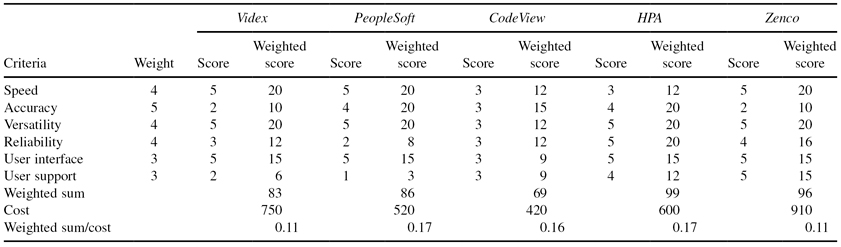
Scoring.
On a scale of 0–5, the maximum weight of 5 was assigned to accuracy—for obvious reasons. The next highest, 4, was assigned to speed, versatility, and reliability, all of which have a direct impact on the utility of the tool. User interface and support were assigned a medium weight of 3 because, while they are important, they are not quite as critical as the others to the successful use of the tool.
Cost was considered separately to enable the consideration of cost/effectiveness as a separate evaluation factor.
The subjective value method was used to determine raw scores. The raw scores for each of the candidates were assigned on a scale of 5 = superior, 4 = good, 3 = satisfactory, 2 = weak, 1 = poor, and 0 = unacceptable. The row below the criteria lists the summed total of the weighted scores. The cost for each candidate tool and the ratio of the total score to the cost are listed in the last two rows.
Analysis.
Comparing the summed scores in Table 9.6 shows that HPA and Zenco score significantly higher than the others. It is worth noting, however, that CodeView scored “satisfactory” on all criteria and is the least expensive by a substantial margin. Videx, CodeView, and HPA are essentially equal in cost/effectiveness.
Sensitivity analysis by varying criteria weightings does not resolve the difference between HPA and Zenco. However, examining the profiles of the candidates’ raw scores highlights the weak performance of Zenco with respect to accuracy. This, coupled with its very high price, would disqualify this candidate. The profile test also highlights the weak reliability and poor user support of PeopleSoft, and the weak accuracy and high price of Videx. In contrast, HPA scores satisfactory or above in all categories and superior in half of them.
The above detailed analysis should result in a recommendation to select HPA as the best tool, with an option of accepting CodeView if cost is a determining factor.
Limitations of Numeric Comparisons
Any decision support method provides information to decision makers; it does not make the decision for them. Stated another way, trade-off analysis is a valuable aid to decision making rather than an infallible formula for success. It serves to organize a set of inputs in a systematical and logical manner, but is wholly dependent on the quality and sufficiency of the inputs.
The above trade-off example illustrates the need for a careful examination of all of the significant characteristics of a trade-off before making a final decision. It is clear that the total candidate scores in themselves mask important information (e.g., the serious weaknesses in some of the candidates). It is also clear that conventional sensitivity analysis does not necessarily suffice to resolve ties or to test the validity of the highest-scoring candidate. The example shows that the decision among alternatives should not be reduced to merely a mathematical exercise.
Furthermore, when, as is very often the case, the relative weightings of MOE are based on qualitative judgments rather than on objective measurements, there are serious implications produced by the automated algorithms that compute the results. One problem is that such methods tend to produce the impression of credibility well beyond the reliability of the inputs. Another is that the results are usually presented to more significant figures than are warranted by the input data. Only in the case of existing products whose characteristics are accurately known are the inputs truly quantitative. For these reasons, it is absolutely necessary to avoid blindly trusting the numbers. A third limitation is that the trade-off studies often fail to include the assumptions that went into the calculations. To alleviate the above problems, it is important to accompany the analysis with a written rationale for the assignment of weighting factors, rounding off the answer to the relevant number of significant figures, and performing a sanity check on the results.
Decision Making
As was stated in the introduction to this section, all important systems engineering decisions should follow the basic principles of the decision-making process. When a decision does not require a report to management, the basic data gathering and reasoning should still be thorough. Thus, all decisions, formal and informal, should be conducted in a systematic manner, use the key requirements to derive the decision criteria, define relevant alternatives, and attempt to compare the candidates’ utility as objectively as practicable. In all important decisions, the opinions of colleagues should be sought to obtain the advantage of collective judgment to resolve complex issues.
9.6 REVIEW OF PROBABILITY
The next section discusses the various evaluation methods that are available to the systems engineer when making decisions among a set of alternatives. All of the evaluation methods involve some level of mathematics, especially probability. Therefore, it is necessary to present a quick review of basic probability theory before describing the methods.
Even in the classical period of history, people noticed that some events could not be predicted with certainty. Initial attempts at representing uncertainty were subjective and nonquantitative. It was not until the late Middle Ages before some quantitative methods were developed. Once mathematics had matured, probability theory could be grounded in mathematical principles. It was not long before probability was applied beyond games of chance and equipossible outcomes (where it started). Before long, probability was applied to the physical sciences (e.g., thermodynamics and quantum mechanics), social sciences (e.g., actuarial tables and surveying), and industrial applications (e.g., equipment failures).
Although modern probability theory is grounded in mathematics, there still exists different perspectives on what probability is and how best it should be used:
- Classical. Probability is the ratio of favorable cases to the total equipossible cases.
- Frequentist. Probability is the limiting value as the number of trials becomes infinite of the frequency of occurrence of a random event that is well-defined.
- Subjectivist. Probability is an ideal rational agent’s degree of belief about an uncertain event. This perspective is also known as Bayesian.
Probability Basics.
At its core, probability is a method of expressing someone’s belief or direct knowledge about the likelihood of an event occurring, or having occurred. It is expressed as a number between zero and one, inclusive. We use the term probability to always refer to uncertainty—that is, information about events that either have yet to occur or have occurred, but our knowledge of their occurrence is incomplete. In other words, probability refers only to situations that contain uncertainty.
As a common example, we can estimate the probability of rain for a certain area within a specified time frame. Typically referred to as “chance,” we commonly hear, “The chance of rain today for your area is 70%.” What does that mean? It actually may have different meanings than is commonly interpreted, unless a precise description is given. However, after the day is over, and it indeed rained for a period of time that day, we cannot say that the probability of rain yesterday was 100%. We do not use probability to refer to known events.
Probability has been described by certain axioms and properties. Some basic properties are provided below:
- 1. The probability of an event, A, occurring is given as a real number between zero and one.
- 2. The probability of an event, A, NOT occurring is represented by several symbols including ∼A,
 A, and A′ (among others), and is expressed as
- 3. The probability of the domain of events occurring (i.e., all possible events) is always
- 4. The probability of the union of two events, A and B, is given by the equation
This concept is depicted in Figure 9.10.
- 5. The probability of an event, A, occurring given that another event, B, has occurred is expressed as P(A|B) and is given by the equation
This concept is depicted in Figure 9.11. In essence, the domain is reduced to the event B, and the probability of the event A is only relevant to the domain of B.
- 6. The probability of the intersection of two events, A and B, is given by the equation

Figure 9.10. Union of two events.

Figure 9.11. Conditional events.
Bayes’ Rule.
Using the above properties and equalities, an important rule was derived by Thomas Bayes (1702–1761). Officially known as Bayes’ theorem, the rule is commonly expressed as the equality
Apart from the mathematical advantages of this rule, a very practical usage of this equality stems from situations that require the conditional relationship among events to reverse. For example, suppose we desire to calculate the probability that a system will fail given that preventative maintenance is performed over a period of time. Unfortunately, we may not have measured data to directly calculate this probability. Suppose that we only have the following probabilities:
- the probability that any system will fail (0.2),
- the probability that a system has had preventative maintenance performed on it over its life cycle (0.4), and
- the probability that a system had preventative maintenance, given it failed (0.02).
How might we calculate the probability that a system will fail, given we perform preventative maintenance over its life cycle? Let us call P(F) as the probability that a system will fail over its life cycle, P(M) as the probability that a system had preventative maintenance over its life cycle, and P(M|F) as the probability that a system had preventative maintenance over its life cycle, given that it failed at some point. This is represented as
We can use Bayes’ rule to calculate the probability we seek:
The probability that our system will fail, given we perform preventative maintenance throughout its life cycle, is very low, 0.013, or almost 20 times lower than the probability of any system failing.
Bayes’ rule is a powerful tool for calculating conditional probabilities. But it does have its limitations. Bayes’ rule assumes that we have a priori knowledge in order to apply it. In most cases, in engineering and science, we either do have a priori knowledge of the domain or can collect data to estimate it. In our example, the a priori knowledge was the probability that any system would fail, P(F). If we did not have this knowledge, then we could not apply Bayes’ rule.
We could collect statistical data on historical system failures to obtain an estimate of P(F). We could also test systems to collect these data. But if the system is new, with new technologies, or new procedures, we may not have sufficient historical data. And applying Bayes’ rule would not be possible.
Now that we have reviewed the basics of probability, we are able to survey and discuss a sample of evaluation methods used in systems engineering today.
9.7 EVALUATION METHODS
In the section above, we described a systematic method for performing trade-off analyses. We used a rather simple scheme for evaluating a set of alternatives against a set of weighted selection criteria. In fact, we used a method that is part of a larger mathematical method, known as multiattribute utility theory (MAUT). Other methods exist that allow systems engineers to evaluate a set of alternatives. Some use a form of MAUT incorporating more complex mathematics to increase accuracy or objectivity, while others take an entirely different approach. This section introduces the reader to five types of methods, commonly used in decision support, starting with a discussion of MAUT. Others exist as well, to include linear programming, integer programming, design of experiments, influence diagrams, and Bayesian networks, to name just a few.
This section is simply an introduction of several, selected mathematical methods. References at the end of this chapter provide sources of more detail on any of these methods.
MAUT
This form of mathematics (which falls under operations research) is used quite extensively in all types of engineering, due to its simplicity. It can easily be implemented via a spreadsheet.
As described above, the basic concept involves identifying a set of evaluation criteria with which to select among a set of alternative candidates. We would like to combine the effectiveness values for these criteria into a single metric. However, these criteria do not have similar meanings that allow their integration. For example, suppose we had three selection criteria: reliability, volume, and weight. How do we evaluate the three together? Moreover, we typically need to trade off one attribute for another. So, how much reliability is worth x volume and y weight? In addition, criteria typically have different units. Reliability has no units as it is a probability; volume may use cubic meter and weight may use kilogram. How do we combine these three criteria into a single measure?
MAUT’s answer to this dilemma is to use the concept of utility and utility functions. A utility function, U(mi), translates the selection criterion, mi, to a unitless measure of utility. This function may be subjective or objective, depending on the data that are available. Typically, utility is measured using a scalar between zero and one, but any range of values will do.
Combining weighted utilities can be accomplished in a number of ways. Three were mentioned above: weighted sum, weighted product, and sum of the logarithms of the weighted utility. Typically, the weighted sum is used, at least as a start. During sensitivity analysis, other methods of combining terms are attempted.
Analytical Hierarchy Process (AHP)
A widely used tool to support decisions in general, and trade studies in particular, is based on the AHP. AHP may be applied using an Excel spreadsheet, or a commercial tool, such as Expert Choice. The latter produces a variety of analyses as well as graphs and charts that can be used to illustrate the findings in the trade study report.
The AHP is based on pairwise comparisons to derive both weighting factors and comparative scores. In deriving criterion-weighting factors, each criterion is compared with every other, and the results are entered into a computation that derives the relative factors. For informal trade-offs, the values obtained by simple prioritization are usually within 10% of those derived by AHP, so the use of the tool is hardly warranted in such cases. On the other hand, for a formal trade study, graphs and charts produced through the use of AHP may lend an appearance of credibility to the presentation.
Weighting factors are calculated using eigenvectors and matrix algebra. Thus, the method has a mathematical basis to it, although the pairwise comparisons are usually subjective, adding uncertainty to the process. The result is a weighting factor distribution among the criteria, summing to one. Figure 9.12 shows the results using the AHP of an example decision to select a new car. Three criteria were used: style, reliability, and fuel economy. After a pairwise comparison among these three criteria, AHP calculated the weights, which sum to one.

Figure 9.12. AHP example.
Once weighting factors are calculated, a second set of pairwise comparisons is performed. These comparisons are among the alternatives, for each criterion. Two results are provided during this stage of the method. First, the alternatives are evaluated within each criterion individually. Each alternative is provided with a criterion score between zero and one, with the sum equal to one. Second, the method produces a final score for each alternative across all criteria, between zero and one, with the sum equal to one. Figure 9.13 displays both sets of results—each alternative car (lettered A through D) is given a score for each criterion, and then the scores are combined into a single, final score.

Figure 9.13. AHP results.
Sensitivity analysis is still needed to check results and to make any changes necessary to arrive at a preferred alternative.
Decision Trees
Decisions were developed to assist decision makers in identifying alternative decision paths and in evaluating and comparing different courses of action. The concept utilizes probability theory to determine the value or utility of alternative decision paths.
As the name suggests, a tree is used to formulate a problem. Typically, two symbols are used—one for decisions and one for events that could occur and are out of the decision maker’s control. Figure 9.14 depicts a simple decision tree in which two decisions and two events are included. The decisions are depicted by rectangles and are lettered A and B; the events are depicted by circles and are designated E1 and E2. In this example, each decision has two possible choices. Events also have more than one outcome, with probabilities associated with each. Finally, the value of each decision path is shown to the right. A value can be anything that represents the quantitative outcome of a decision path. This includes money, production, sales, profit, wildlife saved, and so on.
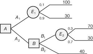
Figure 9.14. Decision tree example.
In this example, an engineer is faced with an initial decision, A. She has two choices, A1 and A2. If she chooses A2, then an event will occur that provides a value to her of either 100 or 30, with a probability of 0.1 or 0.9, respectively. If she chooses A2, she is immediately faced with a second decision, B, which also has two choices, B1 or B2. Choosing B2 will result in a value of 40. Choosing B1 will result in an event, E2, with two possible outcomes. These outcomes result in values of 70 and 30, with probabilities of 0.3 and 0.7, respectively. Which decision path is the “best?”
The answer to the last question is dependent on the objective(s) of the trade-off study. If the study objective is to maximize the expected value of the decision path, then we can solve the tree using a defined method (which we will not go through in detail here). Basically, an analyst or engineer would start at the values (to the right) and work left. First, calculate the expected value for each event. Then at each decision point, choose the greatest expected value. In our example, calculating the events yield an expected value of 37 for E1 and 42 for E2. Thus, decision B is between choosing B1 and gaining a value of 42, over B2, with a value of 40. Decision A is now between two expected values: A1 yields a value of 37, while A2 yields an expected value of 42. Thus, choosing A2 yields the greatest expected value.
The decision tree solution is depicted in Figure 9.15.

Figure 9.15. Decision path.
Of course, the objective may not be to maximize expected value. It may be to minimize expected loss, or to minimize the maximum loss, or even to maximize value. If the objective was the last of these three, maximum value, then choosing A1 would be preferred, since only A1 yields a possibility of achieving a value of 100. Choosing A2 yields a maximum possible value of only 70. Thus, the objective of the trade-off study determines how to solve the tree.
An alternative method of using decision trees is to add a utility assessment. Basically, instead of using values, we use utilities. The reason we may want to substitute utilities for actual values is to incorporate risk into the equation. Suppose, for example, that we have the decision tree shown in Figure 9.16, already solved to maximize the expected value. However, the customer is extremely risk adverse. In other words, the customer would forego larger profits than lose large amounts of value (in this case, the value could be profits).

Figure 9.16. Decision tree solved.
We can develop a utility curve that provides a mathematical representation of the customer’s risk tolerance. Figure 9.17 provides such a curve. The utility curve reveals the customer is conservative—large profits are great, but large losses are catastrophic. Small gains are good, and small losses are acceptable.

Figure 9.17. Utility function.
By substituting utilities for value (in this case, profit), we get a new decision tree and a new solution. The conservative nature of the customer, reflected by the utility curve, reveals a conservative decision path: A2–B2, which yield a utility of 5, which is a profit of 20. Figure 9.18 provides the new decision tree.
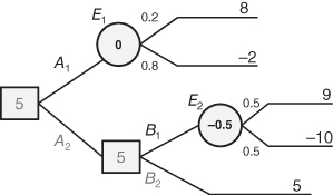
Figure 9.18. Decision tree solved with a utility function.
Decision trees are powerful tools for decision makers to make trade-off decisions. They have the advantage of combining decisions that are interdependent. Although the methods we have discussed can also represent this case, the mathematics becomes more complicated. Their disadvantage includes the fact that a priori knowledge of the event probabilities is required. Methods can be combined—each decision in a decision tree can be represented as a formal trade-off study in itself.
Cost–Benefit Analysis (CBA)
If time and resources permit, a more detailed type of trade-off study can be performed than what is described above. These types of studies are often mandated by policy and are known as an AoA. In many of these situations, the straightforward trade-off study methodology of the last section is not sufficient. Detailed analysis using models, and high-fidelity simulations, are typically required to measure the alternative systems’ effectiveness. In these cases, a CBA is warranted.
The basic concept of the CBA is to measure the effectiveness and estimate the cost of each alternative. These two metrics are then combined in such a way as to shed light on their cost-effectiveness, or put another way, their effectiveness per unit cost. More often than not, the effectiveness of an alternative is a multidimensional metric, and cost is typically divided into its major components: development, procurement, and operations (which include maintenance). In some cases (such as with nuclear reactors), retirement and disposal costs are included.
Combining cost and effectiveness results is crucial in offering decision makers the information they need to make informed decisions. Three basic types of cost-effectiveness analyses exist, each offering advantages. Figure 9.19 illustrates the three types for a single-dimensional analysis.

Figure 9.19. Example of cost-effectiveness integration.
Equal Cost–Variable Effectiveness.
This type constrains the alternatives to a single cost level or a maximum cost threshold. If all of the alternatives are constrained to similar or the same costs, then the results offer an observable difference in effectiveness—enabling a simple ranking of alternatives. In essence, cost is taken out of the equation in comparing alternative systems.
The disadvantages of this CBA include the difficulty in constraining the alternatives to the same, or a maximum cost. Examples include selecting a system within a cost range, such as selecting a new car or purchasing equipment. Of course, one could argue that decisions such as these do not need detailed analysis—a straightforward trade-off study would be sufficient! More detailed examples include a new strike weapon system for the military. A maximum cost level is typically included in a new system’s requirements, including its key performance parameter (KPP). All alternatives are required to be less than the cost threshold. Only effectiveness of these system alternatives varies.
Variable Cost–Equal Effectiveness.
This type constrains the alternatives to a single effectiveness level or a minimum effectiveness threshold. If all of the alternatives are constrained to similar or the same effectiveness levels, then the results offer an observable difference in cost, enabling a simple ranking of alternatives. In essence, effectiveness is taken out of the equation in comparing alternative systems.
The disadvantages of this CBA include the difficulty in constraining the alternatives to the same or minimum effectiveness level. Examples include selecting a power plant to provide a selected amount of energy. In this case, the energy level, or amount of electricity, would be the minimum effectiveness threshold. Options would then be judged largely on cost.
Variable Cost–Variable Effectiveness.
This type constrains the alternatives to both a maximum cost level and a minimum effectiveness level. However, beyond the limits, the alternatives can be any combination of cost and effectiveness. In some cases, no limits are established, and the alternatives are “free” to be at any cost and effectiveness levels. This is rare for government CBAs, but there can be advantages to this form of analysis. Out-of-the-box alternatives can be explored when cost and effectiveness constraints are removed. In some cases, a possible alternative that provides effectiveness that is just under the minimum (say, 5% under the threshold) may cost 50% less than any other alternative. Would not a decision maker at least want to be informed of that possibility? By and large, however, minimum and maximum levels are established to keep the number of alternatives manageable, with the exceptional case being handled separately.
The disadvantages of this CBA type include the risk that no alternative is clearly “better” than the rest. Each alternative offers effectiveness that is commensurate with its cost. Of course, this is not necessarily bad; the decision maker then must decide which alternative he wants. In these cases, calculating the effectiveness per unit cost is an additional measure that can shed light on the decision.
Most systems fall into this category: a new vehicle design, a new spaceship or satellite, a new software system, a new energy system, and so on.
Of course, the examples and notional Figure 9.19 all address single-dimensional applications. Multidimensional costs and effectiveness increase the complexity but still fall into one of the three types of CBA. Two general methods for handling multidimensional CBA are (1) combining effectiveness and cost into a single metric, typically by employing MAUT, then applying one of the three methods described; or (2) using an effectiveness and cost profile vector, with mathematical constraints on the vector as opposed to a single scalar threshold.
Quality Function Deployment (QFD)
QFD originated in Japan during the 1960s as a quality improvement program. Dr. Yoji Akao pioneered the modern version of QFD in 1972 with his article in the journal Standardization and Quality Control, followed by a book describing the process in 1978. Ford Motor Company brought the process to America by adopting it in the 1980s. By the 1990s, some agencies within the U.S. government had adopted the process as well.
At the heart of the process is the QFD matrix, known as the house of quality. Figure 9.20 depicts the general form of this tool, which consists of six elements. More complex forms of the QFD house of quality are also available but are not presented here. The basic use of QFD is in the design process—keeping design engineers, manufacturers, and marketers focused on customer requirements and priorities. It has also been used in decision making.

Figure 9.20. QFD house of quality.
QFD is an excellent tool for developing design objectives that satisfy key customer priorities. It has also been used in trade studies as a method for developing selection criteria and weightings. The output of the house of quality process and analysis is a technical evaluation of alternative subsystems and the relative importance and technical difficulty of developing and manufacturing each component in the technical description. This output is at the bottom of the figure. This evaluation is accomplished by comparing prioritized customer requirements with technical component options and by determining the characteristics of their relationships. Generally, a subset of relationship types, or strengths, is determined. In the figure, four distinct relationships are given: strong, medium, weak, and negative. Additionally, each technical component is compared against other components using the same relationship scale (represented by the triangle at the top or roof of the house). The mathematics (which are not described here but are based on matrix algebra) are then used to determine the technical evaluation.
QFD is typically used in conjunction with trade studies—either to generate inputs to a formal trade study or to conduct the trade studies as part of a design development effort.
9.8 SUMMARY
Decision Making
Decision making is a process that contains several steps. How formal each step is undertaken depends on the type and complexity of the decision. We define a decision framework that examines three types of decisions: structured, semistructured, and unstructured. This categorization is not discrete as the three distinct types suggest but represents a continuum of decisions from the typical/common/understood structured decisions to the atypical/intuitive/subjective unstructured decisions.
The decision-making process has been defined and understood for a long time with little revision. The process contains four phases: preparation and research, model design and evaluation, choosing among alternatives, and implementation.
Modeling throughout System Development
Modeling guides decisions in the face of complexity and uncertainty; modeling illuminates the behavior and relationships of key issues. One modeling tool, simulation, is the modeling of dynamic behavior. Other tools, such as trade-off analysis techniques, model the decision process among alternative choices.
Modeling for Decisions
Models may be divided into three categories.
- 1. Schematic Models use diagrams to represent system elements or processes. An architect’s sketches, such as floor layouts, are examples of schematic models. System block diagrams model system organizations. They are often arranged in a treelike structure to represent hierarchical organizations, or they use simple rectangular boxes to represent physical or other elements.
System context diagrams show all external entities that interact with the system, where the system is represented as a “black box” (not showing internal structure). The diagram describes the system’s interactions with its environment.
FFBDs model functional interactions, where functional elements are represented by rectangles, and arrows represent interactions and flow of information, material, or energy between elements. The names of the elements begin with a verb, denoting action. Examples and extensions of FFBDs include system life cycle models, IDEF0 diagrams, and F2D2.
FFPDs are similar—they form a hierarchical description of a complex process. They also interrelate process design with requirements and specifications.
The diagrams defined by UML and Systems Modeling Language (SysML) are examples of schematic models (see Chapter 8).
- 2. Mathematical Models use mathematical notation to represent relationships. They are important aids to system development and can be useful both for design and systems engineering. They also perform sanity checks on results of complex analyses and simulations.
- 3. Physical Models are physical representations of systems or system elements. They are extensively used in system design and testing, and include test models, mock-ups, and prototypes.
Simulation
System simulations deal with the dynamic behavior of systems and system elements and are used in every phase of system development. Management of simulation effort is a systems engineering responsibility.
Computer “war games” are an example of operational simulations, which involve a simulated adversarial system operated by two teams of players. They are used to assess the operational effectiveness of tactics and system variants.
System effectiveness simulations assess alternative system architectures and are used during conceptual development to make comparative evaluations. The design of effectiveness simulations is itself a complex systems engineering task. Developing complex simulations such as these must seek a balance between fidelity and cost since such simulations can be systems in their own right. Scope must be controlled to obtain effective and timely results.
Physical or physics-based simulations are used in the design of high-performance vehicles and other dynamic systems, and they can save enormous amounts of development time and cost.
Hardware-in-the-loop simulations include hardware components coupled to computer-driven mechanisms. They are a form of physical simulation, modeling dynamic operational environments.
Environmental simulations subject systems and system elements to stressful conditions . They generate synthetic system environments that test systems’ conformance to operational requirements.
Finally, computer-based engineering tools greatly facilitate circuit design, structural analysis, and other engineering functions.
Trade-Off Analysis
Trade-off processes are involved consciously or subconsciously in every decision we make (personally as well as professionally). An important issue with respect to trade studies is the stimulation of alternatives. Trades ultimately select the “best” course of action from two or more alternatives. Major decisions (which are typical within systems engineering) require formal trade-off analysis.
A trade-off, formal or informal, consists of the following steps:
- 1. Define the objective.
- 2. Identify qualified alternative candidates.
- 3. Define selection criteria in the form of MOE.
- 4. Assign weights to selection criteria in terms of their importance to the decision.
- 5. Identify or develop a value rating for each criterion.
- 6. Calculate or collect comparative scores for each alternative’s criterion; combine the evaluations for each alternative.
- 7. Analyze the basis and robustness of the results.
Revise findings if necessary and reject any alternatives that fail to meet an essential requirement. For example, delete MOEs that do not discriminate significantly among alternatives. Limit the value of assignments to the least accurate quantity and examine the total “profile” of scores of the individual candidates.
Trade-off studies and analyses are aids to decision making—they are not infallible formulae for success. Numerical results produce an exaggerated impression of accuracy and credibility. Finally, if the apparent winner is not decisively superior, further analysis is necessary.
Review of Probability
At its core, probability is a method of expressing someone’s belief or direct knowledge about the likelihood of an event occurring or having occurred. It is expressed as a number between zero and one, inclusive. We use the term probability to always refer to uncertainty—that is, information about events that either have yet to occur or have occurred, but our knowledge of their occurrence is incomplete.
Evaluation Methods
As systems engineering is confronted with complex decisions about uncertain outcomes, it has a collection of tools and techniques that can be useful support aids. We present five such tools:
- 1. MAUT uses a utility function to translate a selection criterion to a unitless utility value, which can then be combined with other utility functions to derive a total value score for each alternative.
- 2. AHP is a mathematically based technique that uses pairwise comparisons of criteria and alternatives to general weightings and combines utility scores for alternatives.
- 3. Decision Trees are graphical networks that represent decision choices. Each choice can be assigned a value and an uncertainty measure (in terms of probabilities) to determine expected values of alternative decision paths.
- 4. CBA is a method typically used with modeling and simulation to calculate the effectiveness or a system alternative per unit cost.
- 5. QFD defines a matrix (the house of quality) that incorporates relationships between customers’ needs, system specifications, system components, and component importance to overall design. The matrix can be solved to generate quantitative evaluations of system alternatives.
PROBLEMS
- 9.1 Suppose you needed to make a decision regarding which engine type to use in a new automobile. Using the process in Figure 9.1, describe the five steps in deciding on a new engine type for an advanced automobile.
- 9.2 Identify the stakeholders for the following decisions:
- (a) the design of a traffic light at a new intersection,
- (b) the design of a new weather satellite,
- (c) the choice of a communications subsystem on a new mid-ocean buoy designed to measure ocean temperature at various depths,
- (d) the choice of a security subsystem for a new power plant, and
- (e) the design of a new enterprise management system for a major company.
- 9.3 Give two examples of each decision type: structured, semistructured, and unstructured.
- 9.4 Write an essay describing the purpose of each type of model: schematic, mathematical, and physical. What are their advantages?
- 9.5 Develop a context diagram for a new border security system. This system would be intended to protect the land border between two countries.
- 9.6 In an essay, compare and contrast the three types of functional diagrams: functional block diagram, functional flow diagram, and IDEF0. A table that lists the characteristics of each of the three would be a good start to this problem.
- 9.7 Describe three examples of problems or systems where gaming would be useful in their development and ultimate design.
- 9.8 Perform a trade study on choosing a new car. Identify four alternatives, between three and five criteria, and collect the necessary information required.
- 9.9 To illustrate some important issues in conducting trade studies, consider the following simplified example. The trade study involved six alternative system concepts. Five MOEs were used, each weighted equally. For simplicity’s sake, I have titled the MOEs A, B, C, D, and E. After assigning values to each MOE of the six alternatives, the results were the following:
Note that two stood out well above the rest, both receiving the same total number of points:

On the basis of the above rating profiles,
- (a) Would you conclude that concept III to be superior, equal, or inferior to concept V?
Explain your answer.
- (b) If you were not entirely satisfied with this result, what further information would you try to obtain?
- (c) Discuss potential opportunities for further study that might lead to a clearer recommendation between concepts III and V.
- (a) Would you conclude that concept III to be superior, equal, or inferior to concept V?
- 9.10 Supposed that you are looking to purchase a new vacuum cleaner, and you have decided to conduct a trade study to assist you in your decision. Conduct product research and narrow down your choices to five products.
Please conduct the following steps:
- (a) Identify exactly four selection criteria, not including purchase price or operating cost.
- (b) Assign weights to each criterion, explaining in one sentence your rationale.
- (c) Construct a utility function for each criterion—describe it verbally or graphically.
- (d) Research the actual values for your criteria for each alternative.
- (e) Perform the analysis, calculating a weighted sum for each alternative.
- (f) Calculate the effectiveness/unit cost for each alternative using purchase price for cost.
- (g) Describe your choice for purchase, along with any rationale.
FURTHER READING
R. Clemen and T. Reilly. Making Hard Decisions with DecisionTools Suite. Duxbury Press, 2010.
Defense Acquisition University. Systems Engineering Fundamentals. DAU Press, 2001, Chapter 12.
G. M. Marakas. Decision Support Systems. Prentice Hall, 2001.
C. Ragsdale. Spreadsheet Modeling and Decision Analysis: A Practical Introduction to Management Science. South-Western College Publishing, 2007.
A. P. Sage. Decision Support Systems Engineering. John Wiley & Sons, Inc., 1991.
H. Simon. Administrative Behavior, Third Edition. New York: The Free Press, 1976.
R. H. Sprague and H. J. Watson. Decision Support Systems: Putting Theory into Practice. Prentice Hall, 1993.
E. Turban, R. Sharda, and D. Delan. Decision Support Systems and Intelligence Systems, Ninth Edition. Prentice Hall, 2010.