
6 Teaching machines to see: Image classification with CNNs
- Exploratory data analysis on image data in Python
- Preprocessing and feeding data via image pipelines
- Using the Keras functional API to implement a complex CNN model
- Training and evaluating the CNN model
We have already done a fair bit of work on CNNs. CNNs are a type of network that can operate on two-dimensional data, such as images. CNNs use the convolution operation to create feature maps of images (i.e., a grid of pixels) by moving a kernel (i.e., a smaller grid of values) over the image to produce new values. The CNN has several of these layers that generate more and more high-level feature maps as they get deeper. You can also use max or average pooling layers between convolutional layers to reduce the dimensionality of the feature maps. The pooling layers also move a kernel over feature maps to create the smaller representation of the input. The final feature maps are connected to a series of fully connected layers, where the final layer produces the prediction (e.g., the probability of an image belonging to a certain category).
We have implemented CNN using the Keras Sequential API. We used various Keras layers such as Conv2D, MaxPool2D, and Dense to easily implement CNNs. We’ve already studied various parameters related to the Conv2D and MaxPool2D layers, such as window size, stride, and padding.
In this chapter, we will come a step closer to seeing CNNs performing on real-world data to solve an exciting problem. There’s more to machine learning than implementing a simple CNN to learn from a highly curated data set, as real-world data is often messy. You will be introduced to exploratory data analysis, which is at the heart of the machine learning life cycle. You will explore an image data set, where the objective is to identify the object present in the image (known as image classification). We will then extensively study one of the state-of-the-art models in computer vision, known as the inception model. In deep learning, there are widely recognized neural network architectures (or templates) that perform well on a given task. The inception model is one such model that has been shown to perform well on image data. We will study the architecture of the model and the motivations behind several novel design concepts used in it. Finally, we will train the model on the data set we explored and analyze model performance by relying on metrics such as accuracy on test data.
We have come a long way. We understand the technical aspects of the main deep learning algorithms out there and can be confident in our ability to perform exploratory data analysis correctly and thus enter the model stage with confidence. However, deep networks can get very large very quickly. Complex networks drag in all sorts of computational and performance problems. So, anyone who wants to use these algorithms in real-world problems needs to learn existing models that have proven to perform well in complex learning tasks.
6.1 Putting the data under the microscope: Exploratory data analysis
You are working with a team of data scientists to build a versatile image classification model. The end goal is to use this model as a part of an intelligent shopping assistant. The user can upload a photo of the inside of their home, and the assistant will find suitable products based on their style. The team decided to start out with an image classification model. You need to come back to the group with a great data set to start with and to explain what the data looks like and why it is great. The data set contains day-to-day objects photographed in the real world, and you will do exploratory data analysis and look at various attributes of the data set (e.g., available classes, data set sizes, image attributes) to understand the data and identify and fix potential issues.
Exploratory data analysis (EDA) is the cornerstone of the technical development that you will do in a data science project. The main objective of this process is to get a high-quality clean data set by the end of the process by removing pesky problems like outliers and noise. In order to have such a data set, you need to scrutinize your data and find out if there are
This is by no means an exhaustive list of things to look out for. The more exploration you do, the better the quality of the data.
You have already spent days researching and have found a data set that is appropriate for your problem. To develop an intelligent shopping assistant that can understand customers’ style preferences, it should be able to identify as many household items as possible from the photos that customers will upload. For this, you are planning to use the tiny-imagenet-200 (https://www.kaggle.com/c/tiny-imagenet) data set.
This data set has images belonging to 200 different classes. Figure 6.1 depicts images for some of the available classes.

Figure 6.1 Some sample images from the tiny-imagenet-200. You can see that these images belong to a wide variety of categories.
First things first. We need to download the data set. The following code will create a directory called data in your working directory, download the zip file containing the data, and extract it for you. Finally, you should have a folder called tiny-imagenet-200 in the data folder:
import os
import requests
import zipfile
if not os.path.exists(os.path.join('data','tiny-imagenet-200.zip')):
    url = "http:/ /cs231n.stanford.edu/tiny-imagenet-200.zip"
    r = requests.get(url)

    if not os.path.exists('data'):
        os.mkdir('data')

    with open(os.path.join('data','tiny-imagenet-200.zip'), 'wb') as f:
        f.write(r.content)

    with zipfile.ZipFile(
        os.path.join('data','tiny-imagenet-200.zip'), 'r'
    ) as zip_ref:
        zip_ref.extractall('data')
else:
    print("The file already exists.")
6.1.1 The folder/file structure
The data should now be available in the Ch06/data folder. Now it’s time to explore the data set. The first thing we will do is manually explore the data in the folders provided to us. You’ll note that there are three folders and two files (figure 6.2). Look around and explore them.

Figure 6.2 The folders and files found in the tiny-imagenet-200 data set
The file wnids.txt contains a set of 200 IDs (called wnids or WordNet IDs, based on the lexical database WordNet [https://wordnet.princeton.edu/]; figure 6.3). Each of these IDs represents a single class of images (e.g., class of gold fish).
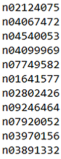
Figure 6.3 Sample content from wnids.txt. It contains wnids (WordNet IDs), one per line.
The file words.txt provides a human touch to these IDs by giving the description of each wnid in a tab-separated-value (TSV) format (table 6.1). Note that this file contains more than 82,000 lines (well over the 200 classes we have) and comes from a much larger data set.
Table 6.1 Sample content from words.txt. It contains the wnids and their descriptions for the data found in the data set.
The train folder contains the training data. It contains a subfolder called images, and within that, you can find 200 folders, each with a label (i.e., a wnid). Inside each of these subfolders, you’ll find a collection of images representing that class. Each subfolder having a wnid as its name contains 500 images per class, 100,000 in total (in all subfolders). Figure 6.4 depicts this structure, as well as some of the data found in the train folder.

Figure 6.4 The overall structure of the tiny-imagenet-200 data set. It has three text files (wnids.txt, words.txt, and val/val_annotations.txt) and three folders (train, val, and test). We will only use the train and val folders.
The val folder contains a subfolder called images and a collection of images (these are not divided into further subfolders like in the train folder). The labels (or wnids) for these images can be found in the val_annotations.txt file in the val folder.
The final folder is called the test folder, which we will ignore in this chapter. This data set is part of a competition, and the data is used to score the submitted models. We don’t have labels for this test set.
6.1.2 Understanding the classes in the data set
We have seen what kind of data we have and where it is available. For the next step, let’s identify some of the classes in the data. For that, we will define a function called get_tiny_imagenet_classes() that reads the wnids.txt and words.txt files and creates a pd.DataFrame (a pandas DataFrame) with two columns: the wnid and its corresponding class description (see the next listing).
Listing 6.1 Getting class descriptions of the classes in the data set
import pandas as pd                                                      ❶
import os                                                                ❶

data_dir = os.path.join('data', 'tiny-imagenet-200')                     ❷
wnids_path = os.path.join(data_dir, 'wnids.txt')                         ❷
words_path = os.path.join(data_dir, 'words.txt')                         ❷

def get_tiny_imagenet_classes(wnids_path, words_path):                   ❸
    wnids = pd.read_csv(wnids_path, header=None, squeeze=True)           ❹
    words = pd.read_csv(words_path, sep='	', index_col=0, header=None)  ❹
    words_200 = words.loc[wnids].rename({1:'class'}, axis=1)             ❺
    words_200.index.name = 'wnid'                                        ❻
    return words_200.reset_index()                                       ❼

labels = get_tiny_imagenet_classes(wnids_path, words_path)               ❽
labels.head(n=25)                                                        ❾
❶ Imports pandas and os packages
❷ Defines paths of the data directory, wnids.txt, and words.txt files
❸ Defines a function to read the class descriptions of tiny_imagenet classes
❹ Reads wnids.txt and words.txt as CSV files using pandas
❺ Gets only the classes present in the tiny-imagenet-200 data set
❻ Sets the name of the index of the data frame to “wnid”
❼ Resets the index so that it becomes a column in the data frame (which has the column name “wnid”)
❽ Executes the function to obtain the class descriptions
❾ Inspects the head of the data frame (the first 25 entries)
This function first reads the wnids.txt that contains a list of wnids that correspond to the classes available in the data set as a pd.Series (i.e., pandas series) object. Next, it reads the words.txt file as a pd.DataFrame (a pandas DataFrame), which contains a wnid to class description mapping, and assigns it to words. Then, it picks the items from words where the wnid is present in the wnids pandas series. This will return a pd.DataFrame with 200 rows (table 6.2). Remember that the number of items in words.txt is much larger than the actual data set, so we only need to pick the items that are relevant to us.
Table 6.2 Sample of the labels’ IDs and their descriptions that we generate using the get_tiny_imagenet_classes() function
We will then compute how many data points (i.e., images) there are for each class:
def get_image_count(data_dir):
    # Get the count of JPEG files in a given folder (data_dir)
    return len(
        [f for f in os.listdir(data_dir) if f.lower().endswith('jpeg')]
    )

   # Apply the function above to all the subdirectories in the train folder
labels["n_train"] = labels["wnid"].apply(
    lambda x: get_image_count(os.path.join(data_dir, 'train', x, 'images'))
)
# Get the top 10 entries in the labels dataframe
labels.head(n=10)
This code creates a new column called n_train that shows how many data points (i.e., images) were found for each wnid. This can be achieved using the pandas pd.Series .apply() function, which applies get_image_count() to each item in the series labels[“wnid”]. Specifically, get_image_count()takes in a path and returns the number of JPEG files found in that folder. When you use this get_image_count() function in conjunction with pd.Series.apply(), it goes to every single folder within the train folder that has a wnid as its name and counts the number of images. Once you run the line labels.head(n=10), you should get the result shown in table 6.3.
Table 6.3 Sample of the data where n_train (number of training samples) has been calculated
Let’s quickly verify that the results are correct. Go into the n02802426 subdirectory in the train folder, which should contain images of basketballs. Figure 6.5 shows a few sample images.

Figure 6.5 Sample images for the wnid category n02802426 (i.e., basketball)
You might find these images quite the opposite of what you expected. You might have expected to see clear and zoomed-in images of basketballs. But in the real world, that’s never the case. Real-life data sets are noisy. You can see the following images:
This will make you admire deep networks a bit more, as this is a hard problem for a bunch of stacked matrix multiplications (i.e., deep networks). Precise scene understanding is required to successfully solve this task. Despite the difficulty, the reward is significant. The model we develop is ultimately going to be used to identify objects in various backgrounds and contexts, such as living rooms, kitchens, and outdoors. And that is exactly what this data set trains your model for: to understand/detect objects in various contexts. You can probably imagine why the modern-day CAPTCHAs are becoming increasingly smarter and can keep up with algorithms that are able to classify objects more accurately. It is not difficult for a properly trained CNN to recognize a CAPTCHA that has cluttered backgrounds or small occlusions.
You can also quickly check the summary statistics (e.g., mean value, standard deviation, etc.) of the n_train column we generated. This provides a more digestible summary of the column than having to look through all 200 rows. This is done using the pandas describe() function:
labels["n_train"].describe()
Executing this will return the following series:
count    200.0
mean     500.0
std        0.0
min      500.0
25%      500.0
50%      500.0
75%      500.0
max      500.0
Name: n_train, dtype: float64
You can see that it returns important statistics of the column, such as the mean value, standard deviation, minimum, and maximum. Every class has 500 images, meaning the data set is perfectly class balanced. This is a handy way to verify that we have a class-balanced data set.
6.1.3 Computing simple statistics on the data set
Analyzing various attributes of the data is also an important step. The type of analysis will change depending on the type of data you work with. Here, we will find out the average size of images (or even the 25/50/75 percentiles).
Having this information ready by the time you get to the actual model saves you a lot of time in making certain decisions. For example, you must know basic statistics of the image size (height and width) to crop or pad images to a fixed size, as image classification CNNs can only process fixed-sized images (see the next listing).
Listing 6.2 Computing image width and height statistics
import os                                                                 ❶
from PIL import Image                                                     ❶
import pandas as pd                                                       ❶

image_sizes = []                                                          ❷
for wnid in labels["wnid"].iloc[:25]:                                     ❸
    img_dir = os.path.join(
        'data', 'tiny-imagenet-200', 'train', wnid, 'images'
    )                                                                     ❹
    for f in os.listdir(img_dir):                                         ❺
        if f.endswith('JPEG'):                                            ❺
            image_sizes.append(Image.open(os.path.join(img_dir, f)).size) ❻

img_df = pd.DataFrame.from_records(image_sizes)                           ❼
img_df.columns = ["width", "height"]                                      ❽
img_df.describe()                                                         ❾
❶ Importing os, PIL, and pandas packages
❷ Defining a list to hold image sizes
❸ Looping through the first 25 classes in the data set
❹ Defining the image directory for a particular class within the loop
❺ Looping through all the images (ending with the extension JPEG) in that directory
❻ Appending the size of each image (i.e., a tuple of (width, height)) to image_sizes
❼ Creating a data frame from the tuples in the image_sizes
❽ Setting column names appropriately
❾ Obtaining the summary statistics of width and height for the images we fetched
Here, we take the first 25 wnids from the labels DataFrame we created earlier (processing all the wnids would take too much time). Then, for each wnid, we go into the subfolder that contains the data belonging to it and obtain the width and height information for each image using
Image.open(os.path.join(img_dir, f)).size
Image.open(<path>).size returns a tuple (width, height) for a given image. We record the width and height of all images we come across in the image_sizes list. Finally, the image_sizes list looks like the following:
image_sizes = [(image_1.width, image_1.height), (image_2.width, image_2.height), ..., (image_n.width, image_n.height)]
For data in this format, we can use the pd.DataFrame.from_records() function to create a pd.DataFrame out of this list. A single element in image_sizes is a record. For example, (image_1.width, image_1.height) is a record. Therefore, image_sizes is a list of records. When you create a pd.DataFrame from a list of records, each record becomes a row in the pandas DataFrame, where each element in each record becomes a column. For example, since we have image width and image height as elements in each record, width and height become columns in the pandas DataFrame. Finally, we execute img_df.describe() to get the basic statistics on the width and height of the images we read (table 6.4).
Table 6.4 Width and height statistics of the images
Next, we will discuss how we can create a data pipeline to ingest the image data we just discussed.
Assume that while browsing through the data set, you came across some corrupted images (i.e., they have negative-valued pixels). Assuming you already have a pd.DataFrame() called df that has a single column with the image file paths (called filepath), use the pandas apply() function to read each image’s minimum value and assign it to a column called minimum. To read the image, you can assume from PIL import Image and import numpy as np have been completed. You can also use np.array(<Image>) to turn a PIL.Image into an array.
6.2 Creating data pipelines using the Keras ImageDataGenerator
You have explored the data set well and understand things like how many classes there are, what kind of objects are present, and the sizes of the images. Now you will create three data generators for three different data sets: training, validation, and test. These data generators retrieve data from the disk in batches and perform any preprocessing required. This way, the data is readily consumable by a model. For this, we will use the convenient tensorflow.keras.preprocessing.image.ImageDataGenerator.
We will start by defining a Keras ImageDataGenerator() to feed in data when we build the model:
from tensorflow.keras.preprocessing.image import ImageDataGenerator
import os

random_seed = 4321
batch_size = 128
image_gen = ImageDataGenerator(samplewise_center=True, validation_split=0.1)
Setting samplewise_center=True, the images generated will have their values normalized. Each image will be centered by subtracting the mean pixel value of that image. validation_split argument plays a vital role in training the data. This lets us split the training data into two subsets, training and validation, by separating a chunk (10% in this example) from the training data. Typically, in a machine learning problem, you should have three data sets:
-
Training data—Typically the largest data set. We use this to train the model.
-
Validation data—Held-out data set. It is not used to train the model but to monitor the performance of the model during training. Note that this validation set must remain fixed (and should not change) during training.
-
Test data—Held-out data set. Unlike the validation data set, this is used only after the training of the model is completed. This represents how well the model will do on unseen real-world data. This is because the model has not interacted with the test data set in any way (unlike the training and validation data sets) until test time.
We will also define a random seed and a batch size for later data generation.
Once you create an ImageDataGenerator, you can use one of its flow functions to read data coming from heterogeneous sources. For example, Keras currently offers the following methods:
-
flow_from_dataframe()—Reads data from a file that contains filenames and their associated labels
-
flow_from_directory()—Reads from a folder where images are organized into subfolders according to the class where they belong
First, we will look at flow_from_directory(), because our train directory is in the exact format flow_from_directory() function expects the data to be in. Specifically, flow_from_directory() expects the data to be in the format shown in figure 6.6.

Figure 6.6 Folder structure expected by the flow_from_directory() method
The flow methods return data generators, which are Python generators. A generator is essentially a function that returns an iterator (called a generator-iterator). But to keep our discussion simple, we will refer to both the generator and the iterator as the generator. You can iterate the generator, just like a list, and return items in a sequential manner. Here’s an example of a generator:
def simple_generator():
    for i in range(0, 100):
        yield (i, i*2)
Note the use of the keyword yield, which you can treat as you do the return keyword. However, unlike return, yield does not exit the function as soon as the line is executed. Now you can define the iterator as
iterator = simple_generator()
You can treat iterator like a list containing [(0, 0), (1, 2), (2, 4), ..., (98, 196), (99, 198)]. However, under the hood, generators are far more memory efficient than list objects. In our case, the data generators will return a single batch of images and targets in a single iteration (i.e., a tuple of images and labels). You can directly feed these generators to a method like tf.keras.models.Model.fit() in order to train a model. The flow_from_directory() method is used to retrieve data:
target_size = (56,56)

train_gen = image_gen.flow_from_directory(
    directory=os.path.join('data','tiny-imagenet-200', 'train'),
    target_size=target_size, classes=None,
    class_mode='categorical', batch_size=batch_size,
    shuffle=True, seed=random_seed, subset='training'
)
valid_gen = image_gen.flow_from_directory (
    directory=os.path.join('data','tiny-imagenet-200', 'train'),
    target_size=target_size, classes=None,
    class_mode='categorical', batch_size=batch_size,
    shuffle=True, seed=random_seed, subset='validation'
)
You can see numerous arguments that have been set for these functions. The most important argument to note is the subset argument, which is set to "training" for train_gen and “validation” for valid_gen. The other arguments are as follows:
-
directory (string)—The location of the parent directory, where data is further divided into subfolders representing classes.
-
target_size (tuple of ints)—Target size of the images as a tuple of (height, width). Images will be resized to the specified height and width.
-
class_mode (string)—The type of targets we are going to provide to the model. Because we want the targets to be one-hot encoded vectors representing each class, we will set it to 'categorical'. Available types include "categorical" (default value), "binary" (for data sets with two classes, 0 or 1), "sparse" (numerical label as opposed to a one-hot encoded vector), "input" or None (no labels), and "raw" or "multi_output" (only available in special circumstances).
-
seed (int)—The random seed for data shuffling, so we get consistent results every time we run it.
-
subset (string)—If validation_split > 0, which subset you need. This needs to be set to either "training" or "validation".
Note that, even though we have 64 × 64 images, we are resizing them to 56 × 56. This is because the model we will use is designed for 224 × 224 images. Having an image size that is a factor of 224 × 224 makes adapting the model to our data much easier.
We can make our solution a bit shinier! You can see that between train_gen and valid_gen, there’s a lot of repetition in the arguments used. In fact, all the arguments except subset are the same for both generators. This repetition clutters the code and creates room for errors (if you need to change arguments, you might set one and forget the other). You can use the partial function in Python to create a partial function with the repeating arguments and then use that to create both train_gen and valid_gen:
from functools import partial
target_size = (56,56)

partial_flow_func = partial(
        image_gen.flow_from_directory,
        directory=os.path.join('data','tiny-imagenet-200', 'train'),
        target_size=target_size, classes=None,
        class_mode='categorical', batch_size=batch_size,
        shuffle=True, seed=random_seed)

train_gen = partial_flow_func(subset='training')
valid_gen = partial_flow_func(subset='validation')
Here, we first create a partial_flow_function (a Python function), which is essentially the flow_from_directory function with some arguments already populated. Then, to create train_gen and valid_gen, we only pass the subset argument. This makes the code much cleaner.
We’re still not done. We need to do a slight modification to the generator returned by the flow_from_directory() function. If you look at an item in the data generator, you’ll see that it is a tuple (x, y), where x is a batch of images and y is a batch of one-hot-encoded targets. The model we use here has a final prediction layer and two additional auxiliary prediction layers. In total, the model has three output layers, so instead of a tuple (x, y), we need to return (x, (y, y, y)) by replicating y three times. We can fix this by defining a new generator data_gen_aux() that takes in the existing generator and modifies its output, as shown. This needs to be done for both the train data generator and validation data generator:
def data_gen_aux(gen):
    for x,y in gen:
        yield x,(y,y,y)

train_gen_aux = data_gen_aux(train_gen)
valid_gen_aux = data_gen_aux(valid_gen)
It’s time to create a data generator for test data. Recall that we said the test data we are using (i.e., the val directory) is structured differently than the train and tran_val data folders. Therefore, it requires special treatment. The class labels are found in a file called val_annotations.txt, and the images are placed in a single folder with a flat structure. Not to worry; Keras has a function for this situation too. In this case, we will first read the val_annotations.txt as a pd.DataFrame using the get_test_labels_df() function. The function simply reads the val_annotations.txt file and creates a pd.DataFrame with two columns, the filename of an image and the class label:
def get_test_labels_df(test_labels_path):
    test_df = pd.read_csv(test_labels_path, sep='	', index_col=None, header=None)
    test_df = test_df.iloc[:,[0,1]].rename({0:"filename", 1:"class"}, axis=1)
    return test_df

test_df = get_test_labels_df(os.path.join('data','tiny-imagenet-200',  'val', 'val_annotations.txt'))
Next, we will use the flow_from_dataframe() function to create our test data generator. All you need to do is pass the test_df we created earlier (for the dataframe argument) and point at the directory where the images can be found (for the directory argument). Note that we are setting shuffle=False for test data, as we would like feed test data in the same order so that the performance metrics we monitor will be the same unless we change the model:
    test_gen = image_gen.flow_from_dataframe(
        dataframe=test_df, directory=os.path.join('data','tiny-imagenet-
➥ 200',  'val', 'images'), target_size=target_size,
➥ class_mode='categorical', batch_size=batch_size, shuffle=False
    )
Next, we are going to define one of the complex computer vision models using Keras and eventually train it on the data we have prepared.
As part of the testing process, say you want to see how robust the model is against corrupted labels in the training data. For this, you plan to create a generator that sets the label to 0 with 50% probability. How would you change the following generator for this purpose? You can use np.random.normal() to draw a value randomly from a normal distribution with zero mean and unit variance:
def data_gen_corrupt(gen):
    for x,y in gen:
        yield x,(y,y,y)
6.3 Inception net: Implementing a state-of-the-art image classifier
You have analyzed the data set and have a well-rounded idea of what the data looks like. For images, you inarguably turn to CNNs, as they are the best in the business. It’s time to build a model to learn customers’ personal tastes. Here, we will replicate one of the state-of-the-art CNN models (known as Inception net) using the Keras functional API.
Inception net is a complex CNN that has made its mark by delivering state-of-the art performance. Inception net draws its name from the popular internet meme “We need to go deeper” that features Leonardo De Caprio from the movie Inception.
The Inception model has six different versions that came out over the course of a short period of time (approximately 2015-2016). That is a testament to how popular the model was among computer vision researchers. To honor the past, we will implement the first inception model that came out (i.e., Inception net v1) and later compare it to other models. As this is an advanced CNN, a good understanding of its architecture and some design decisions is paramount. Let’s look at the Inception model, how is it different from a typical CNN, and most importantly, why it is different.
The Inception model (or Inception net) isn’t a typical CNN. Its prime characteristic is complexity, as the more complex (i.e., more parameters) the model is, the higher the accuracy. For example, Inception net v1 has close to 20 layers. But there are two main problems that rear their heads when it comes to complex models:
-
If you don’t have a big enough data set for a complex model, it is likely the model will overfit the training data, leading to poor overall performance on real-world data.
-
Complex models lead to more training time and more engineering effort to fit those models into relatively small GPU memory.
This demands a more pragmatic way to approach this problem, such as by answering the question “How can we introduce sparsity in deep models (i.e., having fewer parameters) so that the risk of overfitting as well as the appetite for memory goes down?” This is the main question answered in the Inception net model.
Let’s remind ourselves of the basics of CNNs.
6.3.1 Recap on CNNs
CNNs are predominantly used to process images and solve computer vision problems (e.g., image classification, object detection, etc.). As depicted in figure 6.7, a CNN has three components:

Figure 6.7 A simple convolutional neural network. First, we have an image with height, width, and channel dimensions, followed by a convolution and a pooling layer. Finally, the last convolution/pooling layer output is flattened and fed to a set of fully connected layers.
The convolution operation shifts a small kernel (also called a filter) with a fixed size over the width and height dimensions of the input. While doing so, it produces a single value at each position. The convolution operation consumes an input with some width, height, and a number of channels and produces an output that has some width, height, and a single channel. To produce a multichannel output, a convolution layer stacks many of these filters, leading to as many outputs as the number of filters. A convolution layer has the following important parameters:
-
Number of filters—Decides the channel depth (or the number of feature maps) of the output produced by the convolution layer
-
Kernel size—Also known as the receptive field, it decides the size (i.e., height and width) of the filters. The larger the kernel size, the more of the image the model sees at a given time. But larger filters lead to longer training times and larger memory requirements.
-
Stride—Determines how many pixels are skipped while convolving the image. A higher stride leads to a smaller output size (stride is typically used only on height and width dimensions).
-
Padding—Prevents the automatic dimensionality reductions that take place during the convolution operation by adding an imaginary border of zeros, such that the output has the same height and width as the input.
Figure 6.8 shows the working of the convolution operation.
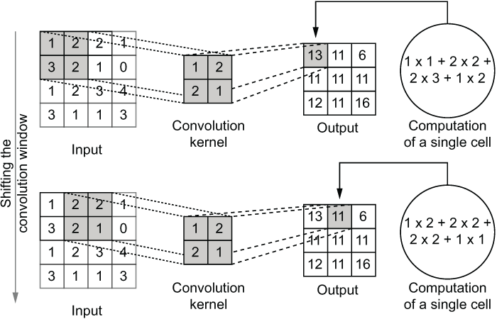
Figure 6.8 The computations that happen in the convolution operation while shifting the window
The pooling operation exhibits the same behavior as the convolution operation when processing an input. However, the exact computations involved are different. There are two different types of pooling: max and average. Max pooling takes the maximum value found in the dark gray box shown in figure 6.9 as the window moves over the input. Average pooling takes the average value of the dark gray box as the window moves over the input.
NOTE CNNs use average pooling as the closest to the output and max pooling layers everywhere else. This configuration has been found to deliver better performance.
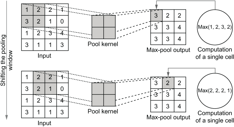
Figure 6.9 How the pooling operation computes the output. It looks at a small window and takes the maximum of the input in that window as the output for the corresponding cell.
The benefit of the pooling operation is that it makes CNNs translation invariant. Translation invariance means that the model can recognize an object regardless of where it appears. Due to the way max pooling is computed, the feature maps generated are similar, even when objects/features are offset by a small number of pixels from what the model was trained on. This means that if you are training a model to classify dogs, the network will be resilient against where exactly the dog appears (only to a certain extent).
Finally, you have a fully connected layer. As we are mostly interested in classification models right now, we need to output a probability distribution over the classes we have for any given image. We do that by connecting a small number of fully connected layers to the end of the CNNs. The fully connected layers will take the last convolution/pooling output as the input and produce a probability distribution over the classes in the classification problem.
As you can see, CNNs have many hyperparameters (e.g., number of layers, convolution window size, strides, fully connected hidden layer sizes, etc.). For optimal results, they need to be selected using a hyperparameter optimization technique (e.g., grid search, random search).
6.3.2 Inception net v1
Inception net v1 (also called GoogLeNet) (http://mng.bz/R4GD) takes CNNs to another level. It is not a typical CNN and requires more effort to implement compared to a standard CNN. At first glance, Inception net might look a bit scary (see figure 6.10). But there are only a handful of new concepts that you need to grok to understand this model. It’s mostly the repetitive application of those concepts that makes the model sophisticated.
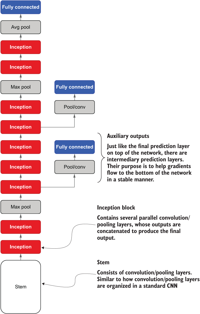
Figure 6.10 Abstract architecture of Inception net v1. Inception net starts with a stem, which is an ordinary sequence of convolution/pooling layers that is found in a typical CNN. Then Inception net introduces a new component known as an Inception block. Finally, Inception net also makes use of auxiliary output layers.
Let’s first understand what’s in the Inception model at a macro level, as shown in figure 6.10, temporarily ignoring the details, such as layers and their parameters. We will flesh these out once we develop a strong macro-level understanding.
Inception net starts with something called a stem. The stem consists of convolution and pooling layers identical to the convolution and pooling layers of a typical CNN. In other words, the stem is a sequence of convolution and pooling layers organized in a specific order.
Next you have several Inception blocks interleaved by max pooling layers. An inception block contains a parallel set of sub-convolution layers with varying kernel sizes. This enables the model to look at the input with different-sized receptive fields at a given depth. We will study the details and motivations behind this in detail.
Finally, you have a fully connected layer, which resembles the final prediction layer you have in a typical CNN. You can also see that there are two more interim fully connected layers. These are known as auxiliary output layers. Just like the final prediction layer, they consist of fully connected layers and a softmax activation that outputs a probability distribution over the classes in the data set. Though they have the same appearance as the final prediction layer, they do not contribute to the final output of the model but do play an important role in stabilizing the model during training. Stable training becomes more and more strenuous as the model gets deeper (mostly due to the limited precision of numerical values in a computer).
Let’s implement a version of the original Inception net from scratch. While doing so, we will discuss any new concepts we come across.
First let’s define a function that creates the stem of Inception net v1. The stem is the first few layers of Inception net and looks like nothing more than the typical convolution/ pooling layers you find in a typical CNN. But there is a new layer (called a lambda layer) that performs something known as local response normalization (LRN). We will discuss the purpose of this layer in more detail soon (see the next listing).
Listing 6.3 Defining the stem of Inception net
def stem(inp):
    conv1 = Conv2D(
        64, (7,7), strides=(1,1), activation='relu', padding='same'
    )(inp)                                                                ❶
maxpool2 = MaxPool2D((3,3), strides=(2,2), padding='same')(conv1)         ❷
lrn3 = Lambda(
    lambda x: tf.nn.local_response_normalization(x)
)(maxpool2)                                                               ❸

conv4 = Conv2D(
    64, (1,1), strides=(1,1), padding='same'
)(lrn3)                                                                   ❹
conv5 = Conv2D(
    192, (3,3), strides=(1,1), activation='relu', padding='same'
)(conv4)                                                                  ❹
    lrn6 = Lambda(lambda x: tf.nn.local_response_normalization(x))(conv5) ❺

    maxpool7 = MaxPool2D((3,3), strides=(1,1), padding='same')(lrn6)      ❻

    return maxpool7                                                       ❼
❶ The output of the first convolution layer
❷ The output of the first max pooling layer
❸ The first local response normalization layer. We define a lambda function that encapsulates LRN functionality.
❹ Subsequent convolution layers
❼ Returns the final output (i.e., output of the max pooling layer)
Most of this code should be familiar to you by now. It is a series of layers, starting from an input to produce an output.
Specifically, we define the following layers:
Going deeper into the Inception block
As stated earlier, one of the main breakthroughs in Inception net is the Inception block. Unlike a typical convolution layer that has a fixed kernel size, the Inception block is a collection of parallel convolutional layers with different kernel sizes. Specifically, the Inception block in Inception v1 contains a 1 × 1 convolution, a 3 × 3 convolution, a 5 × 5 convolution, and pooling. Figure 6.11 shows the architecture of an Inception block.
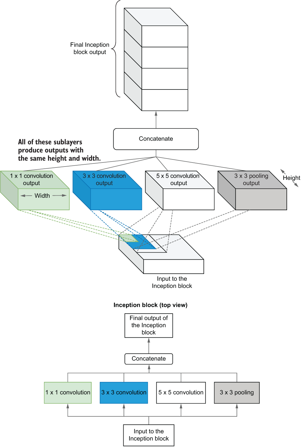
Figure 6.11 The computations in the Inception block, which is essentially a set of parallel convolution/pooling layers with different kernel sizes
Let’s understand why these parallel convolution layers are better than having a giant block of convolution filters with the same kernel size. The main advantage is that the Inception block is highly parameter efficient compared to a single convolution block. We can crunch some numbers to assure ourselves that this is the case. Let’s say we have two convolution blocks: one Inception block and a standard convolution block. Assume that the Inception block has the following:
If you were to design a standard convolution layer that has the representational power of the Inception block, you’d need
Assuming we’re processing an input with a single channel, the inception block has 576 parameters given by
1 × 1 × 1 × 32 + 3 × 3 × 1 × 16 + 5 × 5 × 1 × 16 = 576
The standard convolution block has 1,600 parameters:
In other words, the Inception block has a 64% reduction in the number of parameters compared to a standard convolution layer that has the representational power of the Inception block.
Connection between Inception block and sparsity
For the curious minds out there, there might still be a lingering question: How does the Inception block introduce sparsity? Think of the following two scenarios where you have three convolution filters. In one scenario, you have three 5 × 5 convolution filters, whereas in the other you have a 1 × 1, 3 × 3 and 5 × 5 convolution filter. Figure 6.12 illustrates the difference between the two scenarios.

Figure 6.12 How the Inception block encourages sparsity in the model. You can view a 1 × 1 convolution as a highly sparse 5 × 5 convolution.
It is not that hard to see that when you have three 5 × 5 convolution filters, it creates a very dense connection between the convolution layer and the input. However, when you have a 1 × 1, 3 × 3, and 5 × 5 convolution layer, the connections between the input and the layer are sparser. Another way to think about this is that a 1 × 1 convolution is essentially a 5 × 5 convolution layer, where all the elements are switched off except for the center element. Therefore, a 1 × 1 convolution is a highly sparse 5 × 5 convolution layer. Similarly, a 3 × 3 convolution is a sparse 5 × 5 convolution layer. And by enforcing sparsity, we make the CNN parameter efficient and reduce the chances of overfitting. This explanation is motivated by the discussion found at http://mng.bz/Pn8g.
1 × 1 convolutions as a dimensionality reduction method
Usually, the deeper your model is, the higher the performance (given that you have enough data). As we already know, the depth of a CNN comes at a price. The more layers you have, the more parameters it creates. Therefore, you need to be extra cautious of the parameter count of deep models.
Being a deep model, Inception net leverages 1 × 1 convolution filters within Inception blocks to suppress a large increase in parameters. This is done by using 1 × 1 convolution layers to produce smaller outputs from a larger input and feed those smaller outputs as inputs to the convolution sublayers in the Inception blocks (figure 6.13). For example, if you have a 10 × 10 × 256-sized input, by convolving it with a 1 × 1 convolution layer with 32 filters, you get a 10 × 10 × 32-sized output. This output is eight times smaller than the original input. In other words, a 1 × 1 convolution reduces the channel depth/dimension of large inputs.
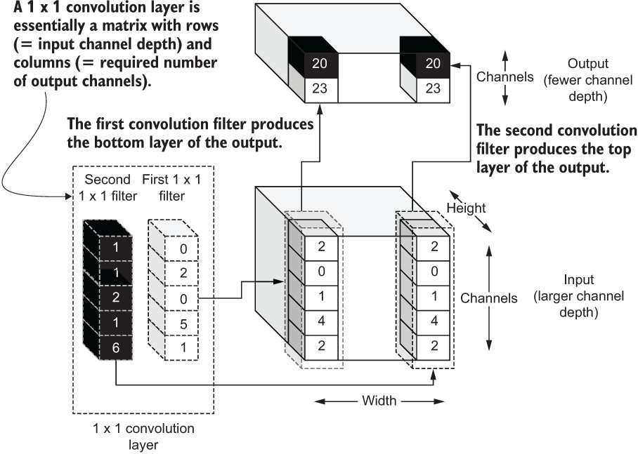
Figure 6.13 The computations of a 1 × 1 convolution and how it enables reduction of a channel dimension of an input
Thus, it is considered a dimensionality reduction method. The weights of these 1 × 1 convolutions can be treated just like parameters of the network and let the network learn the best values for these filters to solve a given task.
Now it’s time to define a function that represents this new and improved Inception block, as shown in the following listing.
Listing 6.4 Defining the Inception block of the Inception net
def inception(inp, n_filters):

    # 1x1 layer
    out1 = Conv2D(
        n_filters[0][0], (1,1), strides=(1,1), activation='relu',
➥ padding='same'
    )(inp)

    # 1x1 followed by 3x3
    out2_1 = Conv2D(
        n_filters[1][0], (1,1), strides=(1,1), activation='relu',
➥ padding='same')
(inp)
    out2_2 = Conv2D(
        n_filters[1][1], (3,3), strides=(1,1), activation='relu',
➥ padding='same'
)(out2_1)

# 1x1 followed by 5x5
out3_1 = Conv2D(
    n_filters[2][0], (1,1), strides=(1,1), activation='relu',
➥ padding='same'
)(inp)
out3_2 = Conv2D(
    n_filters[2][1], (5,5), strides=(1,1), activation='relu',
➥ padding='same'
)(out3_1)

# 3x3 (pool) followed by 1x1
out4_1 = MaxPool2D(
    (3,3), strides=(1,1), padding='same'
)(inp)
out4_2 = Conv2D(
    n_filters[3][0], (1,1), strides=(1,1), activation='relu',
➥ padding='same'
)(out4_1)

out = Concatenate(axis=-1)([out1, out2_2, out3_2, out4_2])
return out
The inception() function takes in some input (four-dimensional: batch, height, width, channel, dimensions) and a list of filter sizes for the convolution sublayers in the Inception block. This list should have the filter sizes in the following format:
[(1x1 filters), (1x1 filters, 3x3 filters), (1x1 filters, 5x5 filters), (1x1 filters)]
The outer loop corresponds to the vertical pillars in the Inception block, and the inner loops correspond to the convolution layers in each pillar (figure 6.14).
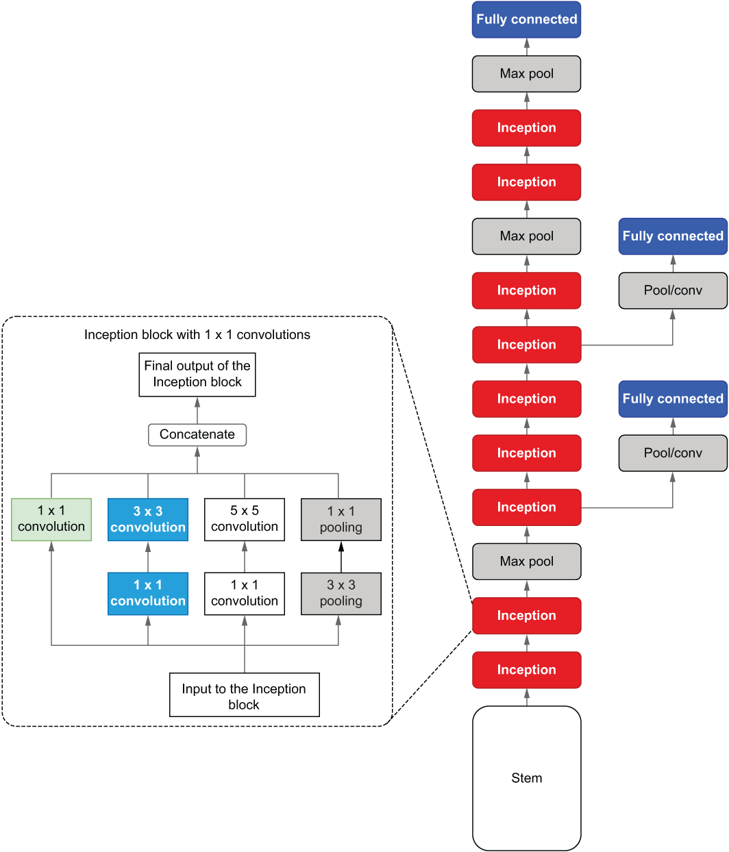
Figure 6.14 The Inception block alongside the full architecture of the Inception net model
We then define the four vertical streams of computations that finally get concatenated to one at the end:
Finally, we concatenate all the outputs of these streams into one on the last axis (denoted by axis = -1). Note the last dimension is the channel dimension of all the outputs. In other words, we are stacking these outputs on the channel dimension. Figure 6.14 illustrates how the Inception block sits in the overall Inception net model. Next, we will discuss another component of the Inception net model known as auxiliary output layers.
Finally, we have two auxiliary output layers that help stabilize our deep CNN. As mentioned earlier, the auxiliary outputs are there to stabilize the training of deep networks. In Inception net, the auxiliary output layer has the following (figure 6.15).
-
A Dense layer with ReLU activation that consumes the flattened output from the 1 × 1 convolution layer
-
A Dense layer with softmax that outputs the probabilities of the classes
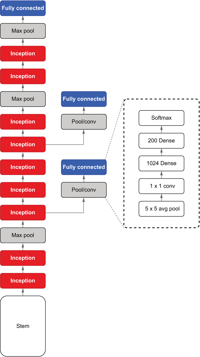
Figure 6.15 Auxiliary output layer alongside the full Inception net architecture
We define a function that produces the auxiliary output predictions as follows (listing 6.5).
Listing 6.5 Defining the auxiliary output as a Python function
def aux_out(inp,name=None):
    avgpool1 = AvgPool2D((5,5), strides=(3,3), padding='valid')(inp)       ❶
    conv1 = Conv2D(128, (1,1), activation='relu', padding='same')(avgpool1)❷
    flat = Flatten()(conv1)                                                ❸
    dense1 = Dense(1024, activation='relu')(flat)                          ❹
    aux_out = Dense(200, activation='softmax', name=name)(dense1)          ❺
    return aux_out
❶ The output of the average pooling layer. Note that it uses valid pooling, which results in a 4 × 4-sized output for the next layer.
❷ 1 × 1 convolution layer’s output
❸ Flattens the output of the convolution layer so that it can be fed to a Dense layer
❹ The first Dense layer’s output
❺ The final prediction for Dense layer’s output
The aux_out() function defines the auxiliary output layer. It starts with an average pool layer with a kernel size of (5,5) and strides (3,3) and valid padding. This means that the layer does not try to correct for the dimensionality reduction introduced while pooling (as done in same padding). Then it’s followed by a convolution layer with 128 filters, (1,1) kernel size, ReLU activation, and same padding. Then, a Flatten() layer is needed before feeding the output to a Dense layer. Remember that the Flatten() layer flattens the height, width, and channel dimension to a single dimension. Finally, a Dense layer with 200 nodes and a softmax activation is applied. With that, we have all the building blocks to build our very own Inception net.
6.3.3 Putting everything together
We have come a long way. Let’s catch our breath and reflect on what we have achieved so far:
-
The abstract architecture and components of the Inception net model consist of a stem, Inception blocks, and auxiliary outputs.
-
Precise details of these components. Stem resembles the stem (everything except the fully connected layers) of a standard CNN. The Inception blocks carry sub-convolution layers with different kernel sizes that encourage sparsity and reduce overfitting.
-
The auxiliary outputs make the network training smoother and rid the network of any undesirable numerical errors during training.
We also defined methods to encapsulate these so that we can call these methods and build the full Inception net. Now we can define the full Inception model (see the next listing). Additionally, you can find the exact Inception block specifications (as per the original paper) summarized in table 6.5.
Listing 6.6 Defining the full Inception net model
def inception_v1():

    K.clear_session()

    inp = Input(shape=(56,56,3))                                          ❶
    stem_out = stem(inp)                                                  ❷
    inc_3a = inception(stem_out, [(64,),(96,128),(16,32),(32,)])          ❸
    inc_3b = inception(inc_3a, [(128,),(128,192),(32,96),(64,)])          ❸

    maxpool = MaxPool2D((3,3), strides=(2,2), padding='same')(inc_3b)

    inc_4a = inception(maxpool, [(192,),(96,208),(16,48),(64,)])          ❸
    inc_4b = inception(inc_4a, [(160,),(112,224),(24,64),(64,)])          ❸

    aux_out1 = aux_out(inc_4a, name='aux1')                               ❹

    inc_4c = inception(inc_4b, [(128,),(128,256),(24,64),(64,)])
    inc_4d = inception(inc_4c, [(112,),(144,288),(32,64),(64,)])
    inc_4e = inception(inc_4d, [(256,),(160,320),(32,128),(128,)])

    maxpool = MaxPool2D((3,3), strides=(2,2), padding='same')(inc_4e)

    aux_out2 = aux_out(inc_4d, name='aux2')                               ❹

    inc_5a = inception(maxpool, [(256,),(160,320),(32,128),(128,)])
    inc_5b = inception(inc_5a, [(384,),(192,384),(48,128),(128,)])
    avgpool1 = AvgPool2D((7,7), strides=(1,1), padding='valid')(inc_5b)   ❺

    flat_out = Flatten()(avgpool1)                                        ❻
    out_main = Dense(200, activation='softmax', name='final')(flat_out)   ❼

    model = Model(inputs=inp, outputs=[out_main, aux_out1, aux_out2])
    model.compile(loss='categorical_crossentropy',
                       optimizer='adam', metrics=['accuracy'])            ❽
    return model
❶ Defines an input layer. It takes a batch of 64 × 64 × 3-sized inputs.
❷ To define the stem, we use the previously defined stem() function.
❸ Defines Inception blocks. Note that each Inception block has different numbers of filters.
❺ The final pooling layer is defined as an Average pooling layer.
❻ The Flatten layer flattens the average pooling layer and prepares it for the fully connected layers.
❼ The final prediction layer that has 200 output nodes (one for each class)
❽ When compiling the model, we use categorical cross-entropy loss for all the output layers and the optimizer adam.
You can see that the model has nine Inception blocks following the original paper. In addition, it has the stem, auxiliary outputs, and a final output layer. The specifics of the layers are listed in table 6.5.
Table 6.5 Summary of the filter counts of the Inception modules in the Inception net v1 model. C(nxn) represents a nxn convolution layer, whereas MaxP(mxm) represents a mxm max-pooling layer.
The layer definitions will be quite similar to what you have already seen. However, the way we define the model and the compilation will be new to some of you. As we discussed, Inception net is a multi-output model. You can define the Keras model with multiple outputs by passing a list of outputs instead of a single output:
model = Model(inputs=inp, outputs=[out_main, aux_out1, aux_out2])
When compiling the model, you can define loss as a list of a single string. If you define a single string, that loss will be used for all the outputs. We compile the model using the categorical cross-entropy loss (for both the final output layer and auxiliary outputs) and the optimizer adam, which is a state-of-the-art optimizer widely used to optimize models and that can adapt the learning rate appropriately as the model trains. In addition, we will inspect the accuracy of the model:
model.compile(loss='categorical_crossentropy', optimizer='adam', metrics=['accuracy'])
With the inception_v1() function defined, you can create a model as follows:
model = inception_v1()
Let’s take a moment to reflect on what we have achieved so far. We have downloaded the data, dissected it, and analyzed the data to understand the specifics. Then we created an image data pipeline using tensorflow.keras.preprocessing.image.ImageDataGenerator. We split the data into three parts: training, validation, and testing. Finally, we defined our model, which is a state-of-the art image classifier known as Inception net. We will now look at other Inception models that have emerged over the years.
6.3.4 Other Inception models
We successfully implemented an Inception net model, which covers most of the basics we need to understand other Inception models. There have been five more Inception nets since the v1 model. Let’s go on a brief tour of the evolution of Inception net.
We have already discussed Inception net v1 in depth. The biggest breakthroughs introduced in Inception net v1 are as follows:
-
The concept of an Inception block, which allows the CNN to have different receptive fields (i.e., kernels sizes) at the same depth of the model. This encourages sparsity in the model, leading to fewer parameters and fewer chances of overfitting.
-
With the 20 layers in the Inception model, the memory of a modern GPU can be exhausted if you are not careful. Inception net mitigates this problem by using 1 × 1 convolution layers to reduce output channel depth whenever it increases too much.
-
The deeper the networks are, the more they are prone to having instable gradients during model training. This is because the gradients must travel a long way (from the top to the very bottom), which can lead to instable gradients. Auxiliary output layers introduced in the middle of the network as regularizers alleviate this problem, leading to stable gradients.
Inception net v2 came not long after Inception net v1 was released (“Rethinking the Inception Architecture for Computer Vision,” https://arxiv.org/pdf/1512.00567.pdf). The main contributions of this model are as follows.
A representational bottle neck occurs when a layer does not have enough capacity (i.e., parameters) to learn a good representation of the input. This can happen if you decrease the size of the layers too fast as you go deep. Inception v2 rejigged the architecture to ensure that no representational bottlenecks are present in the model. This is mostly achieved by changing the layer sizes while keeping the rest of the details the same.
Minimizing the parameters of the network further to reduce overfitting was reinforced. This is done by replacing higher-order convolutions (e.g., 5 × 5 and 7 × 7) with 3 × 3 convolutions (also known as factorizing large convolution layers). How is that possible? Let me illustrate that for you (figure 6.16).

Figure 6.16 A 5 × 5 convolution layer (left) with two 3 × 3 convolution layers (right)
By representing 5 × 5 convolution with two smaller 3 × 3 convolution operations, we enjoy a reduction of 28% in parameters. Figure 6.17 contrasts Inception v1 block with Inception v2 block.
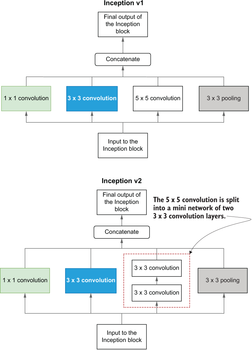
Figure 6.17 Inception block in Inception net v1 (left) versus Inception block in Inception net v2 (right)
Here’s what the TensorFlow code looks like:
# 1x1 layer
out1 = Conv2D(64, (1,1), strides=(1,1), activation='relu', padding='same')(inp)
# 1x1 followed by 3x3
out2_1 = Conv2D(
    96, (1,1), strides=(1,1), activation='relu', padding='same'
)(inp)
out2_2 = Conv2D(
    128, (3,3), strides=(1,1), activation='relu', padding='same'
)(out2_1)

# 1x1 followed by 5x5
# Here 5x5 is represented by two 3x3 convolution layers
out3_1 = Conv2D(
    16, (1,1), strides=(1,1), activation='relu', padding='same'
)(inp)
out3_2 = Conv2D(
    32, (3,3), strides=(1,1), activation='relu', padding='same'
)(out3_1)
out3_3 = Conv2D(
    32, (3,3), strides=(1,1), activation='relu', padding='same'
)(out3_2)

# 3x3 (pool) followed by 1x1
out4_1 = MaxPool2D((3,3), strides=(1,1), padding='same')(inp)
out4_2 = Conv2D(
    32, (1,1), strides=(1,1), activation='relu', padding='same'
)(out4_1)

out = Concatenate(axis=-1)([out1, out2_2, out3_3, out4_2])
But we don’t have to stop here. We can factorize any n × n convolution operation to two 1 × n and n × 1 convolution layers, for example, giving 33% parameter reduction for a 3 × 3 convolution layer (figure 6.18). Empirically, it has been found that factorizing n × n operation to two 1 × n and n × 1 operations is useful only in higher layers. You can refer to the paper to understand when and where these types of factorizations are used.

Figure 6.18 A 3 × 3 convolution layer (left) with 3 × 1 and 1 × 3 convolution layers (right)
Inception v3 was introduced in the same paper as Inception net v2. The primary contribution that sets v3 apart from v2 is the use of batch normalization layers. Batch normalization (“Batch Normalization: Accelerating Deep Network Training by Reducing Internal Covariate Shift,” http://proceedings.mlr.press/v37/ioffe15.pdf) normalizes the outputs of a given layer x by subtracting the mean (E(x)) and standard deviation (√(Var(x)) from the outputs:

This process helps the network stabilize its output values without letting them become too large or too small. Next, it has two trainable parameters, γ and β, that scale and offset the normalized output:
This way, the network has the flexibility to learn its own variation of the normalization by learning optimal γ and β in case x̂ is not the optimal normalization configuration. At this time, all you need to understand is that batch normalization normalizes the output of a given layer in the network. We will discuss how batch normalization is used within the Inception net model in more detail in the next chapter.
Inception-v4 was introduced in the paper “Inception-v4, Inception-ResNet and the Impact of Residual Connections on Learning” (http://mng.bz/J28P) and does not introduce any new concepts, but rather focuses on making the model simpler without sacrificing performance. Mainly, v4 simplifies the stem of the network and other elements. As this is mostly grooming the network’s hyperparameters for better performance and not introducing any new concepts, we will not dive into this model in great detail.
Inception-ResNet v1 and Inception-ResNet v2
Inception-ResNet v1 and v2 were introduced in the same paper and were its main contributions. Inception-ResNet simplifies the Inception blocks that are used in the model and removes some cluttering details. More importantly, it introduces residual connections. Residual connections (or skip connections) were introduced in the paper by Kaiming He et al. titled “Deep Residual Learning for Image Recognition” (https://arxiv.org/ pdf/1512.03385.pdf). It’s an elegantly simple concept, yet very powerful, and it has been responsible for many of the top-performing models in many different domains.
As shown in figure 6.19, residual connections represent simply adding a lower input (close to the input) to a higher-level input (further from the input). This creates a shortcut between the lower input and a higher input, essentially creating another shortcut from the resulting output to the lower layer. We will not dive into too much detail here, as we will discuss Inception-ResNet models in detail in the next chapter. Next, we will train the model we just defined on the image data we have prepared.

Figure 6.19 How residual connections are introduced to a network. It is a simple operation, where you add a lower output (closer to input) of a layer to a higher output (further from input). Skip connections can be designed in such a way to skip any number of layers you like. The figure also highlights the flow of gradients; you can see how skip connections allow gradients to bypass certain layers and travel to lower layers.
As a part of research, you are testing a new technique called poolception. Conceptually similar to an Inception block, poolception has three parallel pooling layers with the following specifications:
Finally, the outputs of these layers are concatenated on the channel axis. Can you implement this as a Python function called poolception that takes the previous layer’s input x as an argument?
6.4 Training the model and evaluating performance
Great work! You have defined one of the state-of-the-art model architectures that has delivered great performance on similar (and larger) data sets. Your next task is to train this model and analyze its performance.
Model training is an imperative step if you need a model that performs well once it’s time to use it. Training the model optimizes (i.e., changes) the parameters of the model in such a way that it can produce the correct prediction given an input. Typically, model training is done for several epochs, where each epoch can consist of thousands of iterations. This process can take anywhere from hours to even weeks depending on the size of the data set and the model. As we have already discussed, deep neural networks, due to their well-known memory requirements, consume data in small batches. A step where the model is optimized with a single data batch is known as an iteration. When you traverse the full data set in such batches, it’s known as an epoch.
Finally, once the training is done, you need to ensure that the model performs well on unseen data. This unseen data must not have had any interaction with the model during the training. The most common evaluation metric for deep learning networks is accuracy. Therefore, we measure the test accuracy to ensure the model’s sturdiness.
In order to train the model, let us first define a function that computes the number of steps or iterations per epoch, given the size of the data set and batch size. It’s always a good idea to run for a predefined number of steps for every epoch. There can be instances where Keras is unable to figure out the number of steps, in which case it can leave the model running until you stop it:
def get_steps_per_epoch(n_data, batch_size):
    if n_data%batch_size==0:
        return int(n_data/batch_size)
    else:
        return int(n_data*1.0/batch_size)+1
It’s a very simple calculation. The number of steps for an epoch is the number of data points (n_data) divided by batch size (batch_size). And if n_data is not divisible by batch_size, you need to add 1 to the returned value to make sure you’re not leaving any data behind. Now let’s train the model in the following listing.
Listing 6.7 Training the Inception net
from tensorflow.keras.callbacks import CSVLogger
import time
import os

if not os.path.exists('eval'):
    os.mkdir('eval')                                               ❶

csv_logger = CSVLogger(os.path.join('eval','1_eval_base.log'))     ❷

history = model.fit(
    x=train_gen_aux,                                               ❸
    validation_data=valid_gen_aux,                                 ❸
    steps_per_epoch=get_steps_per_epoch(0.9*500*200,batch_size),   ❸
    validation_steps=get_steps_per_epoch(0.1*500*200,batch_size),  ❸
    epochs=50,
    callbacks=[csv_logger]                                         ❸
)                                                                  ❸

if not os.path.exists('models'):
    os.mkdir("models")
model.save(os.path.join('models', 'inception_v1_base.h5'))         ❹
❶ Creates a directory called eval to store the performance results
❷ This is a Keras callback that you pass to the fit() function. It writes the metrics data to a CSV file.
❸ By fitting the model, you can see that we are passing the train and validation data generators to the function.
❹ Saves the model to disk so it can be brought up again if needed
When training the model, the following steps are generally followed:
-
At the end of every training epoch, measure performance on the validation data set.
-
After all the training epochs have finished, measure the performance on the test set.
When model.fit() is called in the code, it takes care of the first two steps. We will look at the model.fit() function in a bit more detail. We pass the following arguments to the function:
-
X—Takes the train data generator to the model, which contains both inputs (x) and targets (y).
-
y—Typically takes in the targets. Here we do not specify y, as x already contains the targets.
-
steps_per_epoch—Number of steps (iterations) per epoch in training.
-
validation_steps—Number of steps (iterations) per epoch in validation.
-
callbacks—Any callbacks that need to be passed to the model (for a full list of callbacks visit http://mng.bz/woEW).
You should get something like the following after training the model:
Train for 704 steps, validate for 79 steps
Epoch 1/50
704/704 [==============================] - 196s 279ms/step - loss: 14.6223
➥ - final_loss: 4.9449 - aux1_loss: 4.8074 - aux2_loss: 4.8700 -
➥ final_accuracy: 0.0252 - aux1_accuracy: 0.0411 - aux2_accuracy: 0.0347
➥ - val_loss: 13.3207 - val_final_loss: 4.5473 - val_aux1_loss: 4.3426 -
➥ val_aux2_loss: 4.4308 - val_final_accuracy: 0.0595 - val_aux1_accuracy:
➥ 0.0860 - val_aux2_accuracy: 0.0765
...
Epoch 50/50
704/704 [==============================] - 196s 279ms/step - loss: 0.6361 -
➥ final_loss: 0.2271 - aux1_loss: 0.1816 - aux2_loss: 0.2274 -
➥ final_accuracy: 0.9296 - aux1_accuracy: 0.9411 - aux2_accuracy: 0.9264
➥ - val_loss: 27.6959 - val_final_loss: 7.9506 - val_aux1_loss: 10.4079 -
➥ val_aux2_loss: 9.3375 - val_final_accuracy: 0.2703 - val_aux1_accuracy:
➥ 0.2318 - val_aux2_accuracy: 0.2361
NOTE On an Intel Core i5 machine with an NVIDIA GeForce RTX 2070 8GB, the training took approximately 2 hours and 45 minutes. You can reduce the training time by cutting down the number of epochs.
Finally, we will test the trained model on the test data (i.e., the data in the val folder). You can easily get the model’s test performance by calling model.evaluate() by passing the test data generator (test_gen_aux) and the number of steps (iterations) for the test set:
model = load_model(os.path.join('models','inception_v1_base.h5'))
test_res = model.evaluate(test_gen_aux, steps=get_steps_per_epoch(200*50,
➥ batch_size))
test_res_dict = dict(zip(model.metrics_names, test_res))
You will get the following output:
196/196 [==============================] - 17s 88ms/step - loss: 27.7303 -
➥ final_loss: 7.9470 - aux1_loss: 10.3892 - aux2_loss: 9.3941 -
➥ final_accuracy: 0.2700 - aux1_accuracy: 0.2307 - aux2_accuracy: 0.2367
We can see that the model reaches around 30% validation and test accuracy and a whopping ~94% training accuracy. This is a clear indication that we haven’t steered clear from overfitting. But this is not entirely bad news. Thirty percent accuracy means that the model did recognize around 3,000/10,000 images in the validation and test sets. In terms of the sheer data amount, this corresponds to 60 classes out of 200.
NOTE An overfitted model is like a student who memorized all the answers for an exam, whereas a generalized model is a student who worked hard to understand concepts that will be tested on the exam. The student who memorized answers will only perform well in the exam and fail in the real world, whereas the student who understood concepts can generalize their knowledge both to the exam and the real world.
Overfitting can happen for a number of reasons:
-
The model architecture is not optimal for the data set we have.
-
More regularization is needed to reduce overfitting, such as dropout and batch normalization.
-
We are not using a pretrained model that has already been trained on similar data.
We are going to address each of these concerns in the next chapter, where it will be exciting to see how much things improve.
If you train a model for 10 epochs with a data set that has 50,000 samples with a batch size of 250, how many iterations would you train the model for? Assuming you are given the inputs as a variable x and labels as a variable y, populate the necessary arguments in model.fit() to train the model according to this specification. When not using a data generator, you can set the batch size using the batch_size argument and ignore the steps_per_epoch argument (automatically inferred) in model.fit().
Summary
-
Exploratory data analysis (EDA) is a crucial step in the machine learning life cycle that must be performed before starting on any modeling.
-
The Keras data generator can be used to read images from disk and load them into memory to train the model.
-
Inception net v1 is one of the state-of-the-art computer vision models for image classification designed for reducing overfitting and memory requirements of deep models.
-
Inception net v1 consists of a stem, several inception blocks, and auxiliary outputs.
-
An Inception block is a layer in the Inception net that consists of several sub-convolution layers with different kernel sizes, whereas the auxiliary output ensures smoothness in model training.
-
When training a model, there are three data sets: training, validation, and test.
-
Typically, we train the model on training data for several epochs, and at the end of every epoch, we measure the performance on the validation set. Finally, after the training has finished, we measure performance on the test data set.
-
A model that overfits is like a student who memorized all the answers for an exam. It can do very well on the training data but will do poorly in generalizing its knowledge to analyze unseen data.
Answers to exercises
def get_img_minimum(path):
    img = np.array(Image.open(path))
    return np.min(img)

df[“minimum”] = df[“filepath”].apply(lambda x: get_img_minimum(x))def data_gen_corrupt(gen):
for x,y in gen:
if np.random.normal()>0:
y = 0
yield x,(y,y,y)
def poolception(x):
    out1 = MaxPool2D(pool_size=(3,3), strides=(2,2), padding=’same’)(x)
    out2 = MaxPool2D(pool_size=(5,5), strides=(2,2), padding=’same’)(out1)
    out3 = AvgPool2D(pool_size=(3,3), strides=(2,2), padding=’same’)(out2)
    out = Concatenate(axis=-1)([out1, out2, out3])
    return out
Exercise 4: Total number of iterations = (data set size/batch_size) * epochs = (50,000/250) * 10 = 2,000
model.fit(x=x, y=y, batch_size=250, epochs=10)