
12 Sequence-to-sequence learning: Part 2
- Implementing the attention mechanism for the seq2seq model
- Generating visualizations from the attention layer to glean insights from the model
In the previous chapter, we built an English-to-German machine translator. The machine learning model was a sequence-to-sequence model that could learn to map arbitrarily long sequences to other arbitrarily long sequences. It had two main components: an encoder and a decoder. To arrive at that, we first downloaded a machine translation data set, examined the structure of that data set, and applied some processing (e.g., adding SOS and EOS tokens) to prepare it for the model. Next, we defined the machine translation model using standard Keras layers. A special characteristic of this model is its ability to take in raw strings and convert them to numerical representations internally. To achieve this, we used the Keras’s TextVectorization layer. When the model was defined, we trained it using the data set we processed and evaluated it on two metrics: per-word accuracy of the sequences produced and BLEU. BLEU is a more advanced metric than accuracy that mimics how a human would evaluate the quality of a translation. To train the model, we used a technique known as teacher forcing. When teacher forcing is used, we feed the decoder, with the target translation offset by 1. This means the decoder predicts the next word in the target sequence given the previous word(s), instead of trying to predict the whole target sequence without any knowledge of the target sequence. This leads to better performance. Finally, we had to redefine our model to suit inference. This is because we had to modify the decoder such that it predicted one word at a time instead of a sequence. This way, we can create a recursive decoder at inference time, which predicts a word and feeds the predicted word as an input to predict the next word in the sequence.
In this chapter, we will explore ways to increase the accuracy of our model. To do that, we will use the attention mechanism. Without attention, machine translation models rely on the last output produced after processing the input sequence. Through the attention mechanism, the model is able to obtain rich representations from all the time steps (while processing the input sequence) during the generation of the translation. Finally, we will conclude the chapter by visualizing the attention mechanisms that will give insights into how the model pays attention to words provided to it during the translation process.
The data and the processing we do in this chapter are going to be identical to the last chapter. Therefore, we will not discuss data in detail. You have been provided all the code necessary to load and process data in the notebook. But let’s refresh the key steps we performed:
-
Download the data set manually from http://www.manythings.org/anki/deu-eng.zip.
-
The data is in tab-separated format and <German phrase><tab><English phrase><tab><Attribution> format. We really care about the first two tab-separated values in a record. We are going to predict the German phrase given the English phrase.
-
We randomly sample 50,000 data points from the data set and use 5,000 (i.e., 10%) as validation data and another 5,000 (i.e., 10%) as test data.
-
We add a start token (e.g., SOS) and an end token (e.g., EOS) to each German phrase. This is an important preprocessing step, as this helps us to recursively infer words from our recursive decoder at inference time (i.e., provide SOS as the initial seed and keep predicting until the model outputs EOS or reaches a maximum length).
-
We look at summary statistics of vocabulary size and sequence length, as these hyperparameters are very important for our TextVectorization layer (the layer can be found at tensorflow.keras.layers.experimental.preprocessing.TextVectorization).
-
The vocabulary size is set as the number of unique words that appear more than 10 times in the corpus for both languages, and the sequence length is set as the 99% quantile (plus a buffer of 5) for both languages.
12.1 Eyeballing the past: Improving our model with attention
You have a working prototype of the translator but still think you can push the accuracy up by using attention. Attention provides a richer output from the encoder to the decoder by allowing the decoder to look at all the outputs produced by the encoder over the entire input sequence. You will modify the previously implemented model to incorporate an attention layer that takes all the encoder outputs (one for each time step) and produces a sequence of outputs for each decoder step that will be concatenated with the standard output produced by the decoder.
We have a working machine translator model that can translate from English to German. Performance of this model can be pushed further using something known as Bahdanau attention. Bahdanau attention was introduced in the paper “Neural Machine Translation by Jointly Learning to Align and Translate” by Bahdanau et al. (https://arxiv.org/pdf/1409.0473.pdf). We already discussed self-attention in chapter 5. The underlying principle between the two attention mechanisms is the same. They both allow the model to get a rich representation of historical/future input in a sequence to facilitate the model in understanding the language better. Let’s see how the attention mechanism can be tied in with the encoder-decoder model we have.
The attention mechanism produces an output for each decoder time step, similar to how the decoder’s GRU model produces an output at each time step. The attention output is combined with the decoder’s GRU output and fed to the subsequent hidden layer in the decoder. The attention output produced at each time step of the decoder combines the encoder’s outputs from all the time steps, which provides valuable information about the English input sequence to the decoder. The attention layer is allowed to mix the encoder outputs differently to produce the output for each decoder time step, depending on which part of the translation the decoder model is working on at a given moment. You should be able to see how powerful the attention mechanism is. Previously, the context vector was the only input from the encoder that was accessible to the decoder. This is a massive performance bottleneck, as it is impractical for the encoder to encode all the information present in a sentence using a small-sized vector.
Let’s probe a bit more to understand the specific computations that transpire during the computation of the attention outputs. Let’s assume that the encoder output at position j (1 < j < Te) is denoted by hj, and the decoder RNN output state at time i (1 < i < Td) is denoted by si ; then the attention output ci for the ith decoding step is computed by


Here, W, U, and v are weight matrices (initialized randomly just like neural network weights). Their shapes are defined in accordance with the dimensionality of hidden representations s and h, which will be discussed in detail soon. In summary, this set of equations, for a given decoder position
-
Computes energy values representing how important each encoder output is for that decoding step using a small fully connected network whose weights are W, U, and v
-
Normalizes energies to represent a probability distribution over the encoder steps
-
Computes a weighted sum of encoder outputs using the probability distribution
12.1.1 Implementing Bahdanau attention in TensorFlow
Unfortunately, TensorFlow does not have a built-in layer to readily use in our models to enable the attention mechanism. Therefore, we will implement an Attention layer using the Keras subclassing API. We will call this the DecoderRNNAttentionWrapper and will have to implement the following functions:
-
__init__—Defines various initializations that need to happen before the layer can operate correctly
-
build()—Defines the parameters (e.g., trainable weights) and their shapes associated with the computation
-
call()—Defines the computations and the final output that should be produced by the layer
The __init__() function initializes the layer with any attributes it requires to operate correctly. In this case, our DecoderRNNAttentionWrapper takes in a cell_fn as the argument. cell_fn needs to be a Keras layer object that implements the tf.keras .layers.AbstractRNNCell interface (http://mng.bz/pO18). There are several options, such as tf.keras.layers.GRUCell, tf.keras.layers.LSTMCell, and tf.keras.layers.RNNCell. In this case, we will use the tf.keras.layers.GRUCell.
Here, we have decided to go with GRU, as the GRU model is a lot simpler than an LSTM (meaning there is reduced training time) but achieves roughly similar results on NLP tasks:
def __init__(self, cell_fn, units, **kwargs):
    self._cell_fn = cell_fn
    self.units = units
    super(DecoderRNNAttentionWrapper, self).__init__(**kwargs)
Next, the build() function is defined. The build function declares the three weight matrices used in the attention computation: W, U and v. The argument input_shape contains the shapes of the inputs. Our input will be a tuple containing encoder outputs and the decoder RNN inputs:
def build(self, input_shape):


    self.W_a = self.add_weight(
        name='W_a',
        shape=tf.TensorShape((input_shape[0][2], input_shape[0][2])),
        initializer='uniform',
        trainable=True
    )

    self.U_a = self.add_weight(
        name='U_a',
        shape=tf.TensorShape((self._cell_fn.units, self._cell_fn.units)),
        initializer='uniform',
        trainable=True
    )

    self.V_a = self.add_weight(
        name='V_a',
        shape=tf.TensorShape((input_shape[0][2], 1)),
        initializer='uniform',
        trainable=True
    )

    super(DecoderRNNAttentionWrapper, self).build(input_shape)
The most important argument to note in the weight definitions is the shape argument. We are defining them so that
-
W_a (representing W) has a shape of [ <encoder hidden size>, <attention hidden size>]
-
U_a (representing U) has a shape of [<decoder hidden size>, <attention hidden size>]
-
V_a (representing v) has a shape of [<attention hidden size>, 1]
Here, the <encoder hidden size> and <decoder hidden size> are the number of units in the final output of the RNN layer of the encoder or the decoder, respectively. We typically keep the encoder and decoder RNN sizes the same to simplify the computations. The <attention hidden size> is a hyperparameter of the layer that can be set to any value and represents the dimensionality of internal computations of the attention. Finally, we define the call() method (see listing 12.1). The call() method encapsulates the computations that take place when the layer is called with inputs. This is where the heavy lifting required to compute the attention outputs happens. At a high level, the attention layer needs to traverse all the encoder inputs (i.e., each time step) for each decoder input.
Listing 12.1 Attention computation in the DecoderRNNAttentionWrapper
def call(self, inputs, initial_state, training=False):

    def _step(inputs, states):
        """ Step function for computing energy for a single decoder state
        inputs: (batchsize * de_in_dim)
        states: [(batchsize * de_latent_dim)]
        """

        encoder_full_seq = states[-1]                                   ❶

        W_a_dot_h = K.dot(encoder_outputs, self.W_a)                    ❷

        U_a_dot_s = K.expand_dims(K.dot(states[0], self.U_a), 1)        ❸

        Wh_plus_Us = K.tanh(W_a_dot_h + U_a_dot_s)                      ❹

        e_i = K.squeeze(K.dot(Wh_plus_Us, self.V_a), axis=-1)           ❺
        a_i = K.softmax(e_i)                                            ❺

        c_i = K.sum(encoder_outputs * K.expand_dims(a_i, -1), axis=1)   ❻

        s, states = self._cell_fn(K.concatenate([inputs, c_i], axis=-1),
➥ states)                                                              ❼

        return (s, a_i), states

   """ Computing outputs """

   encoder_outputs, decoder_inputs = inputs                             ❽

   _, attn_outputs, _ = K.rnn(
        step_function=_step, inputs=decoder_inputs,
➥ initial_states=[initial_state], constants=[encoder_outputs]          ❾
   )

   # attn_out => (batch_size, de_seq_len, de_hidden_size)
   # attn_energy => (batch_size, de_seq_len, en_seq_len)
   attn_out, attn_energy = attn_outputs                                 ❿

   return attn_out, attn_energy
❶ When calling the _step function, we are passing encoder_outputs as a constant, as we need access to the full encoder sequence. Here we access it within the _step function.
❷ Computes S.Wa where S represents all the encoder outputs and S=[s0, s1, ..., si]. This produces a [batch size, en_seq_len, hidden size]-sized output.
❸ Computes hj.Ua, where hj represent the j^{th} decoding step. This produces a [ batch_size, 1, hidden size]-sized output
❹ Computes tanh(S.Wa + hj.Ua). This produces a [batch_size, en_seq_len, hidden size]-sized output
❺ Computes the energies and normalizes them. Produces a [batch_size, en_seq_len] sized output
❻ Computes the final attention output (c_i) as a weighted sum of h_j (for all j), where weights are denoted by a_i. Produces a [batch_size, hidden_size] output
❼ Concatenate sthe current input and c_i and feeds it to the decoder RNN to get the output
❽ The inputs to the attention layer are encoder outputs and decoder RNN inputs.
❾ The K.rnn() function executes the _step() function for every input in the decoder inputs to produce attention outputs for all the decoding steps.
❿ The final output is two-fold: attention outputs of a [batch size, de_seq_len, hidden size]-sized output and attention energies [batch dize, de_seq_len, en_seq_len]-sized outputs
Let’s demystify what’s done in this function. The input to this layer is an iterable of two elements: encoder output sequence (encoder_outputs) and decoder RNN input sequence (decoder_inputs). Next, we use a special backend function of Keras called K.rnn() (http://mng.bz/OoPR) to iterate through these inputs while computing the final output required. In our example, it is called as
_, attn_outputs, _ = K.rnn(
        step_function=_step, inputs=decoder_inputs, initial_states=[initial_state], constants=[encoder_outputs],
   )
Here, it applies the step_function to each time step slice of the inputs tensor. For example, the decoder_inputs is a [<batch size>, <decoder time steps>, <embedding size>]-sized input. Then the K.rnn() function applies the step_function to every [<batch size>, <embedding size>] output for <decoder time steps> number of times. The update this function does is a recurrent update, meaning that it takes an initial state and produces a new state until it reaches the end of the input sequence. For that, initial_states provides the starting states. Finally, we are passing encoder_outputs as a constant to the step_function. This is quite important as we need the full sequence of the encoder’s hidden outputs to compute attention at each decoding step. Within the step_function, constants gets appended to the value of the states argument. So, you can access encoder_outputs as the last element of states.
The _step function does the computations we outlined in listing 12.1 for a single decoder time step. It takes inputs (a slice of the time dimension of the original input) and states (initialized with the initial_states value in the K.rnn() function). Next, using these two entities, the normalized attention energies (i.e., αij) for a single time step are computed (a_i). Following that, c_i is computed, which is a weighted sum of encoder_outputs weighted by a_i. Afterward, it updates the cell_fn (i.e., GRUCell) with the current input and the state. Note that the current input to the cell_fn is a concatenation of the decoder input and c_i (i.e., the weighted sum of encoder inputs). The cell function then outputs the output state along with the next state. We return this information out. In other words, the _step() function outputs the output for that time step (i.e., a tuple of decoder RNN output and normalized energies that computed the weighted sum of encoder inputs) and the next state of the decoder RNN.
Finally, you can obtain the full output of the _step function for all the decoder time steps using the K.rnn() function as shown. We are only interested in the output itself (denoted by attn_outputs) and will ignore the other things output by the function.
The K.rnn() function outputs the following outputs when called:
-
last_output—The last output produced by the _step_function after it reaches the end of the sequence
-
new_states—The last states produced by the step_function after it reaches the end of the sequence
Finally, the call() function produces two outputs:
-
attn_out—Holds all the attention outputs for all the decoding steps
-
attn_energy—Provides the normalized energy values for a batch of data, where the energy matrix for one example contains energy values for all the encoder time steps for every decoder time step
We have discussed the most important functions of the DecoderRNNAttentionWrapper layer. If you want to see the full sub-classed implementation of the DecoderRNNAttentionWrapper, please refer to the code at Ch11/11.1_seq2seq_machine_translation .ipynb.
12.1.2 Defining the final model
When defining the final model, the get_vectorizer() and get_encoder() functions remain identical to what was shown in the previous section. All the modifications required need to happen in the decoder. Therefore, let’s define a function, get_ final_seq2seq_model_with_attention(), that provides us the decoder with Bahdanau attention in place, as shown in the next listing.
Listing 12.2 Defining the final sequence-to-sequence model with attention
def get_final_seq2seq_model_with_attention(n_vocab, encoder, vectorizer):
    """ Define the final encoder-decoder model """

    e_inp = tf.keras.Input(shape=(1,), dtype=tf.string, name='e_input_final')
    fwd_state, bwd_state, en_states = encoder(e_inp)                              ❶

    d_inp = tf.keras.Input(shape=(1,), dtype=tf.string, name='d_input')           ❷

    d_vectorized_out = vectorizer(d_inp)                                          ❸

    d_emb_layer = tf.keras.layers.Embedding(
        n_vocab+2, 128, mask_zero=True, name='d_embedding'                        ❹
    )
    d_emb_out = d_emb_layer(d_vectorized_out)                                     ❹

    d_init_state = tf.keras.layers.Concatenate(axis=-1)([fwd_state, bwd_state])   ❺

    gru_cell = tf.keras.layers.GRUCell(256)                                       ❻
    attn_out, _  = DecoderRNNAttentionWrapper(
        cell_fn=gru_cell, units=512, name="d_attention"
    )([en_states, d_emb_out], initial_state=d_init_state)                         ❼

    d_dense_layer_1 = tf.keras.layers.Dense(512, activation='relu', name='d_dense_1')
    d_dense1_out = d_dense_layer_1(attn_out)                                      ❽

    d_final_layer = tf.keras.layers.Dense(
        n_vocab+2, activation='softmax', name='d_dense_final'
    )
    d_final_out = d_final_layer(d_dense1_out)                                     ❽

    seq2seq = tf.keras.models.Model(
        inputs=[e_inp, d_inp], outputs=d_final_out,                               ❾
        name='final_seq2seq_with_attention'
    )

    return seq2seq
❶ Get the encoder outputs for all the timesteps.
❷ The input is (None,1) shaped and accepts an array of strings.
❸ Vectorize the data (assign token IDs).
❹ Define an embedding layer to convert IDs to word vectors.
❺ Define the initial state to the decoder as the concatenation of the last forward and backward encoder states.
❻ Define a GRUCell, which will then be used for the Attention layer.
❼ Get the attention outputs. The GRUCell is passed as the cell_fn, where the inputs are en_states (i.e., all of the encoder states) and d_emb_out (input to the decoder RNN).
❽ Define the intermediate and final Dense layer outputs.
❾ Define a model that takes encoder and decoder inputs as inputs and outputs the final predictions (d_final_out).
We already have done all the hard work. Therefore, changes to the decoder can be summarized in two lines of code:
    gru_cell = tf.keras.layers.GRUCell(256)
    attn_out, _  = DecoderRNNAttentionWrapper(
        cell_fn=gru_cell, units=512, name="d_attention"
    )(
        [en_states, d_emb_out], initial_state=d_init_state
    )
We first define a GRUCell object with 256 hidden units. Then we define the DecoderRNNAttentionWrapper, where the cell_fn is the GRUCell we defined and units is set to 512. units in the DecoderRNNAttentionWrapper defines the dimensionality of the weights and the intermediate attention outputs. We pass en_states (i.e., encoder output sequence) and d_emb_out (i.e., decoder input sequence to the RNN) and set the initial state as the final state of the encoder (i.e., d_init_state).
Next, as before, we have to define a get_vectorizer() function (see the next listing) to get the English/German vectorizers.
Listing 12.3 Defining the TextVectorizers for the encoder-decoder model
def get_vectorizer(
    corpus, n_vocab, max_length=None, return_vocabulary=True, name=None
):

    """ Return a text vectorization layer or a model """

    inp = tf.keras.Input(shape=(1,), dtype=tf.string, name='encoder_input')❶

    vectorize_layer = tf.keras.layers.experimental.preprocessing.TextVectorization(
        max_tokens=n_vocab+2,                                              ❷
        output_mode='int',
        output_sequence_length=max_length,
        name=name
    )

    vectorize_layer.adapt(corpus)                                          ❸

    vectorized_out = vectorize_layer(inp)                                  ❹

    if not return_vocabulary:
        return tf.keras.models.Model(inputs=inp, outputs=vectorized_out)   ❺
    else:
        return tf.keras.models.Model(
            inputs=inp, outputs=vectorized_out                             ❻
        ), vectorize_layer.get_vocabulary()
❶ Define an input layer that takes a list of strings (or an array of strings).
❷ When defining the vocab size, there are two special tokens, (Padding) and '[UNK]' (OOV tokens), added automatically.
❸ Fit the vectorizer layer on the data.
❹ Get the token IDs for the data fed to the input.
❺ Return only the model, which takes an array of a string and outputs a tensor of token IDs.
❻ Return the vocabulary in addition to the model.
The get_encoder() function shown in the following listing builds the encoder. As these have been discussed in detail, they will not be repeated here.
Listing 12.4 The function that returns the encoder
def get_encoder(n_vocab, vectorizer):
    """ Define the encoder of the seq2seq model"""

    inp = tf.keras.Input(shape=(1,), dtype=tf.string, name='e_input')  ❶

    vectorized_out = vectorizer(inp)                                   ❷


    emb_layer = tf.keras.layers.Embedding(
        n_vocab+2, 128, mask_zero=True, name='e_embedding'             ❸
    )

    emb_out = emb_layer(vectorized_out)                                ❹

    gru_layer = tf.keras.layers.Bidirectional(
        tf.keras.layers.GRU(128, name='e_gru'),                        ❺
        name='e_bidirectional_gru'
    )

    gru_out = gru_layer(emb_out)                                       ❻
    encoder = tf.keras.models.Model(
        inputs=inp, outputs=gru_out, name='encoder'
    )                                                                  ❼

    return encoder
❶ The input is (None,1) shaped and accepts an array of strings.
❷ Vectorize the data (assign token IDs).
❸ Define an embedding layer to convert IDs to word vectors.
❹ Get the embeddings of the token IDs
❺ Define a bidirectional GRU layer. The encoder looks at the English text (i.e., the input) both backward and forward; this leads to better performance.
❻ Get the output of the GRU layer (the last output state vector returned by the model).
❼ Define the encoder model; this takes in a list/array of strings as the input and returns the last output state of the GRU model as the output.
As the very last step, we define the final model and compile it using the same specifications we used for the earlier model:
# Get the English vectorizer/vocabulary
en_vectorizer, en_vocabulary =
➥ get_vectorizer(np.array(train_df["EN"].tolist()), en_vocab, max_length=en_seq_length, name='e_vectorizer')
# Get the German vectorizer/vocabulary
de_vectorizer, de_vocabulary =
➥ get_vectorizer(np.array(train_df["DE"].tolist()), de_vocab,
➥ max_length=de_seq_length-1, name='d_vectorizer')

# Define the final model with attention
encoder = get_encoder_with_attention(en_vocab, en_vectorizer)
final_model_with_attention =
➥ get_final_seq2seq_model_with_attention(de_vocab, encoder, de_vectorizer)

# Compile the model
final_model_with_attention.compile(
    loss='sparse_categorical_crossentropy',
    optimizer='adam',
    metrics=['accuracy']
)
12.1.3 Training the model
Training the model is quite straightforward as it remains the same as before. All we need to do is call the train_model() function with the arguments model (a Keras model to be trained/evaluated), vectorizer (a target language vectorizer to convert token IDs to text), train_df (training data), valid_df (validation data), test_df (testing data), epochs (an int to represent how many epochs the model needs to be trained) and batch_size (size of a training/evaluation batch):
epochs = 5
batch_size = 128

train_model(final_model_with_attention, de_vectorizer, train_df, valid_df,
➥ test_df, epochs, batch_size)Evaluating batch 39/39
Epoch 1/5
(train) loss: 2.096887740951318 - accuracy: 0.6887444907274002 -
➥ bleu: 0.00020170408678925458
(valid) loss: 1.5872839291890461 - accuracy: 0.7375801282051282 -
➥ bleu: 0.002304922518160425
...
Evaluating batch 39/39
Epoch 5/5
(train) loss: 0.7739567615282841 - accuracy: 0.8378756006176655 -
➥ bleu: 0.20010080750506093
(valid) loss: 0.8180131682982812 - accuracy: 0.837830534348121 -
➥ bleu: 0.20100039279462362
Evaluating batch 39/39
(test) loss: 0.8390972828253721 - accuracy: 0.8342147454237326 - bleu:
➥ 0.19782372616582572Compared to the last model we had, this is quite an improvement. We have almost doubled the validation and testing BLEU scores. All this was possible because we introduced the attention mechanism to alleviate a huge performance bottleneck in the encoder-decoder model.
NOTE On an Intel Core i5 machine with an NVIDIA GeForce RTX 2070 8 GB, the training took approximately five minutes to run five epochs.
Finally, for later use, we save the trained model, along with the vocabularies:
## Save the model
os.makedirs('models', exist_ok=True)
tf.keras.models.save_model(final_model_with_attention,
➥ os.path.join('models', 'seq2seq_attention'))

# Save the vocabulary
import json
os.makedirs(
    os.path.join('models', 'seq2seq_attention_vocab'), exist_ok=True
)
with open(os.path.join('models', 'seq2seq_attention_vocab',
➥ 'de_vocab.json'), 'w') as f:
    json.dump(de_vocabulary, f)

with open(os.path.join('models', 'seq2seq_attention_vocab',
➥ 'en_vocab.json'), 'w') as f:
json.dump(en_vocabulary, f)With that, we will discuss how we can visualize the attention weights to see the attention patterns the model uses when decoding inputs.
You have invented a novel attention mechanism called AttentionX. Unlike Bahdanau attention, this attention mechanism takes encoder inputs and the decoder’s RNN outputs to produce the final output. The fully connected layers take this final output instead of the usual decoder’s RNN output. Given that, you’ve implemented the new attention mechanism in a layer called AttentionX. For encoder input x and decoder’s RNN output y, it can be called as
z = AttentionX()([x, y])
where the final output z is a [<batch size>, <decoder time steps>, <hidden size>]-sized output. How would you change the following decoder to use this new attention mechanism?
e_inp = tf.keras.Input(shape=(1,), dtype=tf.string, name='e_input_final')
fwd_state, bwd_state, en_states = encoder(e_inp)

d_inp = tf.keras.Input(shape=(1,), dtype=tf.string, name='d_input')

d_vectorized_out = vectorizer(d_inp)

d_emb_layer = tf.keras.layers.Embedding(
    n_vocab+2, 128, mask_zero=True, name='d_embedding'
)
d_emb_out = d_emb_layer(d_vectorized_out)

d_init_state = tf.keras.layers.Concatenate(axis=-1)([fwd_state, bwd_state])

gru_out = tf.keras.layers.GRU(256, return_sequences=True)(
    d_emb_out, initial_state=d_init_state
)

d_dense_layer_1 = tf.keras.layers.Dense(512, activation='relu', name='d_dense_1')
d_dense1_out = d_dense_layer_1(attn_out)

d_final_layer = tf.keras.layers.Dense(
    n_vocab+2, activation='softmax', name='d_dense_final'
)
d_final_out = d_final_layer(d_dense1_out)
12.2 Visualizing the attention
You have determined that the attention-based model works better than the one without attention. But you are skeptical and want to understand if the attention layer is producing meaningful outputs. For that, you are going to visualize attention patterns generated by the model for several input sequences.
Apart from the performance, one of the lucrative advantages of the attention mechanism is the interpretability it brings along to the model. The normalized energy values, one of the interim outputs of the attention mechanism, can provide powerful insights into the model. Since the normalized energy values represent how much each encoder output contributed to decoding/translating at each decoding timestep, it can be used to generate a heatmap, highlighting the most important words in English that correspond to a particular German word.
If we go back to the DecoderRNNAttentionWrapper, by calling it on a certain input, it produces two outputs:
The second output is what we are after. That tensor holds the key to unlocking the powerful interpretability brought by the attention mechanism.
Let’s write a function called the attention_visualizer() that will load the saved model and outputs not only the predictions of the model, but also the attention energies that will help us generate the final heatmap. In this function, we will load the model and create outputs by using the trained layers to retrace the interim and final outputs of the decoder, as shown in the next listing. This is similar to how we retraced the various steps in the model to create an inference model from the trained model.
Listing 12.5 A model that visualizes attention patterns from input text
def attention_visualizer(save_path):
    """ Define the attention visualizer model """

    model = tf.keras.models.load_model(save_path)                  ❶

    e_inp = tf.keras.Input(
        shape=(1,), dtype=tf.string, name='e_input_final'
    )                                                              ❷
    en_model = model.get_layer("encoder")                          ❷
    fwd_state, bwd_state, en_states = en_model(e_inp)              ❷

    e_vec_out = en_model.get_layer("e_vectorizer")(e_inp)          ❸

    d_inp = tf.keras.Input(
        shape=(1,), dtype=tf.string, name='d_infer_input'
    )                                                              ❹

    d_vec_layer = model.get_layer('d_vectorizer')                  ❺
    d_vec_out = d_vec_layer(d_inp)                                 ❺

    d_emb_out = model.get_layer('d_embedding')(d_vec_out)          ❻

    d_attn_layer = model.get_layer("d_attention")                  ❻

    d_init_state = tf.keras.layers.Concatenate(axis=-1)(
        [fwd_state, bwd_state]
    )                                                              ❻

    attn_out, attn_states = d_attn_layer(
        [en_states, d_emb_out], initial_state=d_init_state
    )                                                              ❻

    d_dense1_out = model.get_layer("d_dense_1")(attn_out)          ❻

    d_final_out = model.get_layer("d_dense_final")(d_dense1_out)   ❻

    visualizer_model = tf.keras.models.Model(                      ❼
        inputs=[e_inp, d_inp],
        outputs=[d_final_out, attn_states, e_vec_out, d_vec_out]
    )

return visualizer_model❷ Define the encoder input for the model and get the final outputs of the encoder.
❸ Get the encoder vectorizer (required to interpret the final output).
❺ Get the decoder vectorizer and the output.
❻ The next few steps just reiterate the steps in the trained model. We simply get the corresponding layers and pass the output of the previous step to the current step.
❼ Here we define the final model to visualize attention patterns; we are interested in the attn_states output (i.e., normalized energy values). We will also need the vectorized token IDs to annotate the visualization.
Note how the final model we defined returns four different outputs, as opposed to the trained model, which only returned the predictions. We will also need a get_ vocabulary() function that will load the saved vocabularies:
def get_vocabularies(save_dir):
    """ Load the vocabularies """

    with open(os.path.join(save_dir, 'en_vocab.json'), 'r') as f:
        en_vocabulary = json.load(f)

    with open(os.path.join(save_dir, 'de_vocab.json'), 'r') as f:
        de_vocabulary = json.load(f)

    return en_vocabulary, de_vocabulary
Finally, call these functions so that we have the vocabularies and the model ready:
print("Loading vocabularies")
en_vocabulary, de_vocabulary = get_vocabularies(
    os.path.join('models', 'seq2seq_attention_vocab')
)

print("Loading weights and generating the inference model")
visualizer_model = attention_visualizer(
    os.path.join('models', 'seq2seq_attention')
)
print("	Done")
Next, we’ll move on to visualizing the outputs produced by the visualizer_model; we will be using the Python library matplotlib to visualize attention patterns for several examples. Let’s define a function called visualize_attention() that takes in the visualizer_model, the two vocabularies, a sample English sentence, and the corresponding German translation (see the next listing). Then it will make a prediction on the inputs, retrieve the attention weights, generate a heatmap, and annotate the two axes with the English/German tokens.
Listing 12.6 Visualizing attention patterns using input text
import matplotlib.pyplot as plt
%matplotlib inline

def visualize_attention(visualizer_model, en_vocabulary, de_vocabulary,
➥ sample_en_text, sample_de_text, fig_savepath):
    """ Visualize the attention patterns """

    print("Input: {}".format(sample_en_text))

    d_pred, attention_weights, e_out, d_out = visualizer_model.predict(
        [np.array([sample_en_text]), np.array([sample_de_text])]
    )                                                              ❶

    d_pred_out = np.argmax(d_pred[0], axis=-1)                     ❷

    y_ticklabels = []                                              ❸
    for e_id in e_out[0]:                                          ❸
        if en_vocabulary[e_id] == "":                              ❸
            break                                                  ❸
        y_ticklabels.append(en_vocabulary[e_id])                   ❸

    x_ticklabels = []                                              ❹
    for d_id in d_pred_out:                                        ❹
        if de_vocabulary[d_id] == 'eos':                           ❹
            break                                                  ❹
        x_ticklabels.append(de_vocabulary[d_id])                   ❹

    fig, ax = plt.subplots(figsize=(14, 14))

    attention_weights_filtered = attention_weights[
        0, :len(y_ticklabels), :len(x_ticklabels)
    ]                                                              ❺

    im = ax.imshow(attention_weights_filtered)                     ❻

    ax.set_xticks(np.arange(attention_weights_filtered.shape[1]))  ❼
    ax.set_yticks(np.arange(attention_weights_filtered.shape[0]))  ❼
    ax.set_xticklabels(x_ticklabels)                               ❼
    ax.set_yticklabels(y_ticklabels)                               ❼

    ax.tick_params(labelsize=20)                                   ❼
    ax.tick_params(axis='x', labelrotation=90)                     ❼

    plt.colorbar(im)                                               ❽
    plt.subplots_adjust(left=0.2, bottom=0.2)

    save_dir, _ = os.path.split(fig_savepath)                      ❾
    if not os.path.exists(save_dir):                               ❾
        os.makedirs(save_dir, exist_ok=True)                       ❾
    plt.savefig(fig_savepath)                                      ❾
❷ Get the token IDs of the predictions of the model.
❸ Our y tick labels will be the input English words. We stop as soon as we see padding tokens.
❹ Our x tick labels will be the predicted German words. We stop as soon as we see the EOS token.
❺ We are going to visualize only the useful input and predicted words so that things like padded values and anything after the EOS token are discarded.
❻ Generate the attention heatmap.
❼ Set the x ticks, y ticks, and tick labels.
❽ Generate the color bar to understand the value range found in the heat map.
❾ Save the figure to the disk.
First, we input the English and German input text to the model to generate a prediction. We need to input both the English and German inputs as we are still using the teacher-forced model. You might be wondering, “Does that mean I have to have the German translation ready and can only visualize attention patterns in the training mode?” Of course not! You can have an inference model defined, like we did in a previous section in this chapter, and still visualize the attention patterns. We are using the trained model itself to visualize patterns, as I want to focus on visualizing attention patterns rather than defining the inference model (which we already did for another model).
Once the predictions and attention weights are obtained, we define two lists: x_ticklabels and y_ticklabels. They will be the labels (i.e., English/German words) you see on the two axes in the heatmap. We will have the English words on the row dimension and German words in the column dimension (figure 12.1). We will also do a simple filtering to get rid of paddings (i.e., "") and German text appearing after the EOS token and get the attention weights within the range that satisfy these two criteria. You can then simply call the matplotlib’s imshow() function to generate the heatmap and set the axes’ ticks and the labels for those ticks. Finally, the figure is saved to the disk.
Let’s give this a trial run! Let’s take a few examples from our test DataFrame and visualize attention patterns. We will create 10 visualizations and will also make sure that those 10 examples we choose have at least 10 English words to make sure we don’t visualize very short phrases:
# Generate attention patterns for a few inputs
i = 0
j = 0
while j<9:
    sample_en_text = test_df["EN"].iloc[i]
    sample_de_text = test_df["DE"].iloc[i:i+1].str.rsplit(n=1,
➥ expand=True).iloc[:,0].tolist()
    i += 1

    if len(sample_en_text.split(" ")) > 10:
        j += 1
    else:
        continue

    visualize_attention(
        visualizer_model, en_vocabulary, de_vocabulary, sample_en_text,
        sample_de_text, os.path.join('plots','attention_{}.png'.format(i))
    )
If you run this code successfully, you should get 10 attention visualizations shown and stored on the disk. In figures 12.1 and 12.2, we show two such visualizations.
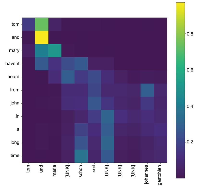
Figure 12.1 Attention patterns visualized for an input English text
In the figures, the lighter the color, the more the model has paid attention to that word. In figure 12.1, we can see that, when translating the words, “und” and “maria,” the model has mostly paid attention to “and” and “mary,” respectively. If you go to Google Translate and do the German translations for the word “and,” for example, you will see that this is, in fact, correct. In figure 12.2, we can see that when generating “hast keine nicht,” the model has paid attention to the phrase “have no idea.” The other observation we can make is that the attention pattern falls roughly diagonally. This makes sense as both these languages roughly follow the same writing style.

Figure 12.2 Attention patterns visualized for an input English text
This concludes our discussion about sequence-to-sequence models. In the next chapter, we will discuss a family of models that has been writing the state-of-the-art of machine learning for a few years: Transformers.
You have an attention matrix given by attention_matrix, with English words given by english_text_labels and German words given by german_text_labels. How would you create a visualization similar to figure 12.1? Here, you will need to use the imshow(), set_xticks(), set_yticks(), set_xticklabels(), and set_yticklabels() functions.
Summary
-
Using attention in sequence-to-sequence models can greatly help shoot their performance up.
-
Using attention at each decoding time step, the decoder gets to see all the historical outputs of the encoder and select and mix these outputs to come up with an aggregated (e.g., summed) representation of that, which gives a holistic view of what was in the encoder input.
-
One of the intermediate products in the attention computation is the normalized energy values, which give a probability distribution of how important each encoded position was for decoding a given time step for every decoding step. In other words, this is a matrix that has a value for every encoder time step and decoder time step combination. This can be visualized as a heatmap and can be used to interpret which words the decoder paid attention to when translating a certain token in the decoder.
Answers to exercises
e_inp = tf.keras.Input(
    shape=(1,), dtype=tf.string, name='e_input_final'
)
fwd_state, bwd_state, en_states = encoder(e_inp)

d_inp = tf.keras.Input(shape=(1,), dtype=tf.string, name='d_input')

d_vectorized_out = vectorizer(d_inp)

d_emb_layer = tf.keras.layers.Embedding(
    n_vocab+2, 128, mask_zero=True, name='d_embedding'
)
d_emb_out = d_emb_layer(d_vectorized_out)

d_init_state = tf.keras.layers.Concatenate(axis=-1)([fwd_state, bwd_state])

gru_out = tf.keras.layers.GRU(256, return_sequences=True)(
    d_emb_out, initial_state=d_init_state
)

attn_out = AttentionX()([en_states, gru_out])

d_dense_layer_1 = tf.keras.layers.Dense(
    512, activation='relu', name='d_dense_1'
)
d_dense1_out = d_dense_layer_1(attn_out)

d_final_layer = tf.keras.layers.Dense(
    n_vocab+2, activation='softmax', name='d_dense_final'
)
d_final_out = d_final_layer(d_dense1_out)im = ax.imshow(attention_matrix)
ax.set_xticks(np.arange(attention_matrix.shape[1]))
ax.set_yticks(np.arange(attention_matrix.shape[0]))
ax.set_xticklabels(german_text_labels)
ax.set_yticklabels(english_text_labels)