
Chapter 32
Managed Futures
Mark J. P. Anson, CFA, Ph.D., CPA, Esq.
Chief Investment Officer CalPERS
Managed futures refers to the active trading of futures contracts and forward contracts on physical commodities, financial assets, and currencies. The purpose of the managed futures industry is to enable investors to profit from changes in futures prices. In this chapter managed futures as an investment vehicle are discussed.
INDUSTRY BASICS
The managed futures industry is another skill-based style of investing. Investment managers attempt to use their special knowledge and insight in buying and selling futures and forward contracts to extract a positive return. These futures managers tend to argue that their superior skill is the key ingredient to derive profitable returns from the futures markets.
There are three ways to access the skill-based investing of the managed futures industry: public commodity pools, private commodity pools, and individual managed accounts. Commodity pools are investment funds that pool the money of several investors for the purpose of investing in the futures markets. They are similar in structure to hedge funds, and are considered a subset of the hedge fund marketplace.
Every commodity pool must be managed by a general partner. Typically, the general partner for the pool must register with the Commodity Futures Trading Commission and the National Futures Association as a Commodity Pool Operator (CPO). However, there are exceptions to the general rule.
Public commodity pools are open to the general public for investment in much the same way a mutual fund sells its shares to the public. Public commodity pools must file a registration statement with the Securities and Exchange Commission before distributing shares in the pool to investors. An advantage of public commodity pools is the low minimum investment and the frequency of liquidity (the ability to cash out).
Private commodity pools are sold to high net worth investors and institutional investors to avoid the lengthy registration requirements of the SEC and sometimes to avoid the lengthy reporting requirements of the CFTC. Otherwise, their investment objective is the same as a public commodity pool. An advantage of private commodity pools is usually lower brokerage commissions and greater flexibility to implement investment strategies and extract excess return from the futures markets.
Commodity pool operators (for either public or private pools) typically hire one or more Commodity Trading Advisors (CTAs) to manage the money deposited in the pool. CTAs are professional money managers in the futures markets.
Like CPOs, CTAs must register with the Commodity Futures Trading Commission (CFTC) and the National Futures Association (NFA) before managing money for a commodity pool. In some cases a managed futures investment manager is registered as both a CPO and a CTA. In this case, the general partner for a commodity pool may also act as its investment adviser.
Last, wealthy and institutional investors can place their money directly with a CTA in an individually managed account. These separate accounts have the advantage of narrowly defined and specific investment objectives as well as full transparency to the investor.
CTAs may invest in both exchange-traded futures contracts and forward contracts. A forward contract has the same economic structure as a futures contract with one difference; it is traded over the counter. Forward contracts are private agreements that do not trade on a futures exchange. Therefore, they can have terms that vary considerably from the standard terms of an exchange-listed futures contracts. Forward contracts accomplish the same economic goal as futures contracts but with the flexibility of custom tailored terms.
HISTORY OF MANAGED FUTURES
Organized futures trading began in the United States in the 1800s with the founding of the Chicago Board of Trade (CBOT) in 1848. It was founded by 82 grain merchants and the first exchange floor was above a flour store. Originally, it was a cash market where grain traders came to buy and sell supplies of flour, timothy seed, and hay.
In 1851, the earliest futures contract in the United States was recorded for the forward delivery of 3,000 bushels of corn, and two years later, the CBOT established the first standard futures contract in corn. Since then, the heart and soul of the CBOT has been its futures contracts on agricultural crops grown primarily in the midwestern states: corn, wheat, and soybeans. Therefore, commodity futures exchanges were founded initially by grain producers and buyers to hedge the price risk associated with the harvest and sale of crops.
Other futures exchanges were established for similar reasons. The Chicago Mercantile Exchange (CME), for example, lists futures contracts on livestock. Chicago was once famous for its stockyards where cattle and hogs were herded to the market. Ranchers and buyers came to the CME to hedge the price risk associated with the purchase and sale of cattle and hogs.
Other exchanges are the New York Mercantile Exchange (NYMEX) where futures contracts on energy products are traded. The Commodity Exchange of New York (now the COMEX division of the NYMEX) lists futures contracts on precious and industrial metals. The New York Coffee, Sugar, and Cocoa Exchange lists futures contracts on (what else?) coffee, sugar, and cocoa. The New York Cotton Exchange lists contracts on cotton and frozen concentrated orange juice.1 The Kansas City Board of Trade lists futures contracts on wheat and financial products such as the Value Line stock index.
Over the years, certain commodities have risen in prominence while others have faded. For instance, the heating oil futures contract was at one time listed as inactive on the NYMEX for lack of interest. For years, heating oil prices remained stable, and there was little interest or need to hedge the price risk of heating oil. Then along came the Arab Oil Embargo of 1973, and this contract quickly took on a life of its own as did other energy futures contracts.
Conversely, other futures contracts have faded away because of minimal input into the economic engine of the United States. For instance, rye futures traded on the CBOT from 1869 to 1970, and barley futures traded from 1885 to 1940. However, the limited importance of barley and rye in finished food products led to the eventual demise of these futures contracts.
As the wealth of America grew, a new type of futures contract has gained importance: financial futures. The futures markets changed dramatically in 1975 when the CBOT introduced the first financial futures contract on Government National Mortgage Association mortgage-backed certificates. This was followed two years later in 1977 with the introduction of a futures contract on the U.S. Treasury Bond. Today this is the most actively traded futures contract in the world.
The creation of a futures contract that was designed to hedge financial risk as opposed to commodity price risk opened up a whole new avenue of asset management for traders, analysts, and portfolio managers. Now, it is more likely that a financial investor will flock to the futures exchanges to hedge her investment portfolio than a grain purchaser will trade to hedge commodity price risk. Since 1975, more and more financial futures contracts have been listed on the futures exchanges. For instance, in 1997 stock index futures and options on the Dow Jones 30 Industrial Companies were first listed on the CBOT. The S&P 500 stock index futures and options (first listed in 1983) are the most heavily traded contracts on the CME. Additionally, currency futures were introduced on the CME in the 1970s (originally listed as part of the International Monetary Market).
With the advent of financial futures contracts more and more managed futures trading strategies were born. However, the history of managed futures products goes back more than 50 years.
The first public futures fund began trading in 1948 and was active until the 1960s. This fund was established before financial futures contracts were invented, and consequently, traded primarily in agricultural commodity futures contracts. The success of this fund spawned other managed futures vehicles, and a new industry was born.
The managed futures industry has grown from just $1 billion under management in 1985 to $35 billion of funds invested in managed futures products in 2000. The stock market’s return to more rational pricing in 2000 helped fuel increased interest in managed futures products. Still, managed futures products are a fraction of the estimated size of the hedge fund marketplace of $400 to $500 billion. Yet, issues of capacity are virtually nonexistent in the managed futures industry compared to the hedge fund marketplace where the best hedge funds are closed to new investors.
Similar to hedge funds, CTAs and CPOs charge both management fees and performance fees. The standard “1 and 20” (1% management fee and 20% incentive fee) are equally applicable to the managed futures industry although management fees can range from 0% to 3% and incentive fees from 10% to 35%.
Unfortunately, until the early 1970s, the managed futures industry was largely unregulated. Anyone could advise an investor as to the merits of investing in commodity futures, or form a fund for the purpose of investing in the futures markets. Recognizing the growth of this industry, and the lack of regulation associated with it, in 1974 Congress promulgated the Commodity Exchange Act (CEA) and created the Commodity Futures Trading Commission (CFTC).
Under the CEA, Congress first defined the terms Commodity Pool Operator and Commodity Trading Advisor. Additionally, Congress established standards for financial reporting, offering memorandum disclosure, and bookkeeping. Further, Congress required CTAs and CPOs to register with the CFTC. Last, upon the establishment of the National Futures Association (NFA) as the designated self-regulatory organization for the managed futures industry, Congress required CTAs and CPOs to undergo periodic educational training.
Today, there are four broad classes of managed futures trading; agricultural products, energy products, financial and metal products, and currency products. Before examining these categories we review the prior research on the managed futures industry.
PRIOR EMPIRICAL RESEARCH
There are two key questions with respect to managed futures:
- Will an investment in managed futures improve the performance of an investment portfolio?
- Can managed futures products produce consistent returns?
The case for managed futures products as a viable investment is mixed. Elton, Gruber, and Rentzler, in three separate studies, examine the returns to public commodity pools.2 In their first study, they conclude that publicly offered commodity funds are not attractive either as standalone investments or as additions to a portfolio containing stocks and/or bonds. In their second study, they find that the historical return data reported in the prospectuses of publicly offered commodity pools are not indicative of the returns that these funds actually earn once they go public. In fact, they conclude that the performance discrepancies are so large that the prospectus numbers are seriously misleading. In their last study, they did not find any evidence that would support the addition of commodity pools to a portfolio of stocks and bonds and that commodity funds did not provide an attractive hedge against inflation. Last, they find that the distribution of returns to public commodity pools to be negatively skewed. Therefore, the opportunity for very large negative returns is greater than for large positive returns.
Irwin, Krukemeyer, and Zulaf,3 Schneeweis, Savanyana, and McCarthy,4 and Edwards and Park5 also conclude that public commodity funds offer little value to investors as either stand-alone investments or as an addition to a stock and bond portfolio. However, Irwin and Brorsen find that public commodity funds provide an expanded efficient investment frontier.6
For private commodity pools, Edwards and Park find that an equally weighted index of commodity pools have a sufficiently high Sharpe Ratio to justify them as either a stand-alone investment or as part of a diversified portfolio.7 Conversely, Schneeweis et al. conclude that private commodity pools do not have value as stand-alone investments but they are worthwhile additions to a stock and bond portfolio.8
With respect to separate accounts managed by CTAs, McCarthy, Schneeweis, and Spurgin9 find that an allocation to an equally weighted index of CTAs provides valuable diversification benefits to a portfolio of stocks and bonds. In a subsequent study, Schneeweis, Spurgin, and Potter find that a portfolio allocation to a dollar weighted index of CTAs results in a higher portfolio Sharpe ratio.10 Edwards and Park find that an index of equally weighted CTAs performs well as both a stand-alone investment and as an addition to a diversified portfolio.11
An important aspect of any investment is the predictability of returns over time. If returns are predictable, then an investor can select a commodity pool or a CTA with consistently superior performance. Considerable time and effort has been devoted to studying the managed futures industry to determine the predictability and consistency of returns. Unfortunately, the results are not encouraging.
For instance, Edwards and Ma find that once commodity funds go public through a registered public offering, their average returns are negative.12 They conclude that prior pre-public trading performance for commodity pools is of little use to investors when selecting a public commodity fund as an investment. The lack of predictability in historical managed futures returns is supported by the research of McCarthy, Schneeweis, and Spurgin;13 Irwin, Zulauf, and Ward;14 and the three studies by Elton, Gruber, and Renzler.15 In fact, Irwin et al conclude that a strategy of selecting CTAs based on historical good performance is not likely to improve upon a naive strategy of selecting CTAs at random.
In summary, the prior research regarding managed futures is unsettled. There is no evidence that public commodity pools provide any benefits either as a stand-alone investment or as part of a diversified portfolio. However, the evidence does indicate that private commodity pools and CTA managed accounts can be a valuable addition to a diversified portfolio. Nonetheless, the issue of performance persistence in the managed futures industry is unresolved. Currently, there is more evidence against performance persistence than there is to support this conclusion.
In the next section, we begin to analyze the performance in the managed futures industry by examining the return distributions for different CTA investment styles. We then consider the potential for downside risk protection from managed futures.
RETURN DISTRIBUTIONS OF MANAGED FUTURES
Similar to our analysis for hedge funds and passive commodity futures, we examine the distribution of returns for managed futures. We use the Barclays Managed Futures Index to determine the pattern of returns associated with several styles of futures investing.
Managed futures products may be good investments if the pattern of their returns is positively skewed. One way to consider this concept is that it is similar to owning a Treasury bill plus a lottery ticket. The investor consistently receives low, but positive returns. However, every once in a while an extreme event occurs and the CTA is able to profit from the movement of futures prices. This would result in a positive skew.
To analyze the distribution of returns associated with managed futures investing, we use the Barclays CTA managed futures indices that divide the CTA universe into four actively traded strategies: (1) CTAs that actively trade in the agricultural commodity futures; (2) CTAs that actively trade in currency futures; (3) CTAs that actively trade in financial and metal futures; and, (4) CTAs that actively trade in energy futures.
Managed futures traders have one goal in mind: to capitalize on price trends. Most CTAs are considered to be trend followers. Typically, they look at various moving averages of commodity prices and attempt to determine whether the price will continue to trend up or down, and then trade accordingly. Therefore, it is not the investment strategy that is the distinguishing factor in the managed futures industry, but rather, the markets in which CTAs and CPOs apply their trend following strategies.16
In this chapter we use the Mount Lucas Management Index (MLMI) as a benchmark by which to judge CTA performance. The MLMI is a passive futures index. It applies a mechanical and transparent rule for capitalizing on price trends in the futures markets. It does not represent active trading. Instead, it applies a consistent rule for buying or selling futures contracts depending upon the current price trend in any particular commodity futures market. In addition, the MLMI invests across agricultural, currency, financial, energy, and metal futures contracts. Therefore, it provides a good benchmark by which to examine the four managed futures strategies.
Exhibit 32.1 shows the distribution of returns for the MLMI. The distribution is negatively skewed. Therefore, a simple or naive trend following strategy will produce a distribution of returns that has more negative return observations below the median than positive observations above the median. In reviewing the distribution of returns for managed futures strategies, we keep in mind that the returns are generated from active management. One demonstration of skill is the ability to shift a distribution of returns from a negative skew to a positive skew. Therefore, if CTAs do in fact have skill, we would expect to see distribution of returns with a positive skew.
Further, the passive MLMI strategy produces a distribution of returns with considerable leptokurtosis. This indicates that the tails of the distribution have greater probability mass than a normal, bell-shaped distribution. This indicates that a passive trend following strategy has significant exposure to outlier events. Consequently, we would expect to observe similar leptokurtosis associated with managed futures.
Last, the average return for the MLMI strategy was 0.73% per month. If managed futures strategies can add value, we would expect them to outperform the average monthly return earned by the naive MLMI strategy.

EXHIBIT 32.1 Distribution of Returns for the MLMI
Managed Futures in Agricultural Commodities
In our discussion of commodity futures in Chapter 10, we indicated that commodity prices are more likely to be susceptible to positive price surprises. The reason is that most of the news associated with agricultural products is usually negative. Droughts, floods, storms, and crop freezes are the main news stories. Therefore, new information to the agricultural market tends to result in positive price shocks instead of negative price shocks. (There is not much price reaction to the news that “the crop cycle is progressing normally.”) We would expect the CTAs to capture the advantage of these price surprises and any trends that develop from them.
Exhibit 32.2 presents the return distribution for Barclays Agricultural CTA index. We use data over the period 1990–2000. From a quick review of this distribution, it closely resembles a bell curve type of distribution. However, in Exhibit 32.6, we show that this distribution in fact has a positive skew of 0.18. Therefore, compared to the negative skew observed for the passive MLMI, we can conclude that managed futures did add value compared to a passive strategy.
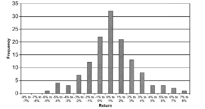
EXHIBIT 32.2 Barclays Agricultural CTA Returns
In addition, the value of kurtosis, while still positive at 0.69, is much smaller than that for the MLMI. In fact, the tails of the distribution for the Barclays Agricultural CTA index have probability mass close to that for a normal distribution. Therefore, CTAs were able to shift the distribution of commodity futures returns from a negative skew to a positive skew while reducing the exposure to tail risk.
Unfortunately, there is a tradeoff for this skill. The average return to the Barclays Agricultural CTA index of 0.58% per month is less than that for the MLMI index of 0.73%. Additionally, the Sharpe ratio for the managed futures strategy is lower than that for the MLMI. Consequently, the results for managed futures trading in the agriculture markets is mixed. On the one hand, we observe a positive shift to the distribution of returns, but on the other, a reduction in the risk and return tradeoff as measured by the Sharpe ratio.
Managed Futures in Currency Markets
The currency markets are the most liquid and efficient markets in the world. The reason is simple, every other commodity, financial asset, household good, cheeseburger, and so on must be denominated in a currency. As the numeraire, currency is the commodity in which all other commodities and assets are denominated.
Daily trading volume in exchange-listed and forward markets for currency contracts is in the hundreds of billions of dollars. Given the liquidity, depth, and efficiency of the currency markets, we would expect the ability of managed futures traders to derive value to be small.
Exhibit 32.3 provides the distribution of returns for actively managed currency futures. We can see from this graph and later in Exhibit 32.6, that CTAs produced a distribution of returns with a very large positive skew of 1.39. This is considerably greater than that for the MLMI, and presents a strong case for skill. In addition, the average monthly return for CTAs trading in currency futures is 0.8% per month, an improvement of the average monthly return for the MLMI.

EXHIBIT 32.3 Barclays Currency CTA Returns
Unfortunately, this strategy also provides a higher value of kurtosis, 3.15, indicating significant exposure to outlier events. This higher exposure to outlier events translates into a higher standard deviation of returns for managed currency futures, and a lower Sharpe ratio.
The evidence for skill-based investing in managed currency futures is mixed. On the one hand, CTAs demonstrated an ability to shift the distribution of returns compared to a naive trend following strategy from negative to positive. On the other hand, more risk was incurred through greater exposure to outlier events resulting in a lower Sharpe ratio than that for the MLMI.
Managed Futures in the Financials and Metals Markets
As we discussed, with the advent of the GNMA futures contract in the 1970s, financial futures contracts have enjoyed greater prominence than traditional physical commodity futures. However, considerable liquidity exists in the precious metals markets because gold, silver, and platinum are still purchased and sold primarily as a store of value rather than for any productive input into a manufacturing process. In this fashion, precious metal futures resemble financial assets.
Financial assets tend to have a negative skew of returns during the period 1990–2000 with a reasonably large value of leptokurtosis. Therefore, a demonstration of skill with respect to managed futures is again the ability to shift the distribution of returns to a positive skew.
Exhibits 32.4 and 32.5 demonstrate this positive skew. Managed futures in financial and precious metal futures have a positive skew of 0.58 and a small positive kurtosis of 0.49. Therefore, CTAs were able to shift the distribution of returns to the upside while reducing exposure to outlier returns.

EXHIBIT 32.4 Barclays Financial and Metals CTA Returns

EXHIBIT 32.5 Barclays Energy CTA Returns
The average monthly return, however, is 0.63%, less than that for the MLMI. Additionally, the Sharpe ratio for this CTA strategy is less than that for the MLMI. Once again, we find mixed evidence that managed futures can add value beyond that presented in a mechanical trend following strategy.
Managed Futures in the Energy Markets
The energy markets are chock full of price shocks associated with news events. These news events tend to be positive for the price of energy related commodities and futures contracts thereon. The Arab Oil Embargo in 1973 and 1977, the Iraq/Iran war of the early 1980s, the Iraqi invasion of Kuwait in 1990, as well as sudden cold snaps, broken pipelines, oil refinery fires and explosions, and oil tanker shipwrecks all tend to increase the price of oil and oil related products.
If there is skill in the managed futures industry with respect to energy futures contracts, we would expect to see a positively skewed distribution with a large expected return. In addition, we would expect to see a large value of kurtosis that reflects the exposure to these outlier events.
Exhibits 32.5 and 32.6 present the results for managed futures in the energy markets.17 The results are consistent with our expectations for skew and kurtosis. CTAs did manage to produce a positively skewed distribution of returns. Additionally, a large value of leptokurtosis is observed, consistent with the energy price shocks that affect this market in particular.
| MLMI | CTA Agriculture |
CTA Currency |
CTA Financial |
CTA Energy |
|
| Expected Return | 0.73% | 0.58% | 0.80% | 0.63% | ‒0.06% |
| Standard Deviation | 1.61% | 2.33% | 3.58% | 2.21% | 5.55% |
| Sharpe Ratio | 0.173 | 0.055 | 0.098 | 0.081 | ‒0.091 |
| Skew | ‒0.562 | 0.182 | 1.394 | 0.587 | 0.309 |
| Kurtosis | 2.476 | 0.693 | 3.147 | 0.491 | 14.616 |
EXHIBIT 32.6 Return Distributions for Managed Futures
Yet, the average return for managed futures in the energy markets is a ‒0.06% per month. Therefore, even though CTAs are able to shift the distribution of returns to a positive skew, the distribution is centered around a negative mean return. While a positive skew to a distribution is a favorable characteristic of any asset class, it has no utility to an investor if the asset class still loses money. Therefore, we must conclude that managed futures in the energy markets did little to add value for an investor.
Given the mixed and disappointing results observed in Exhibits 32.2 through 32.6, we explore another possible use for managed futures: downside risk protection. We examine this prospect in the next section.
MANAGED FUTURES AS DOWNSIDE RISK PROTECTION FOR STOCKS AND BONDS
The greatest concern for any investor is downside risk. If equity and bond markets are becoming increasingly synchronized, international diversification may not offer the protection sought by investors. The ability to protect the value of an investment portfolio in hostile or turbulent markets is the key to the value of any macroeconomic diversification.
Within this framework, an asset class distinct from financial assets has the potential to diversify and protect an investment portfolio from hostile markets. It is possible that “skill-based” strategies such as managed futures investing can provide the diversification that investors seek. Managed futures strategies might provide diversification for a stock and bond portfolio because the returns are dependent upon the special skill of the CTA rather than any macroeconomic policy decisions made by central bankers or government regimes.
Exhibit 32.7 presents the return distribution for a portfolio that was 60% the S&P 500 and 40% U.S. Treasury bonds. Our concern is the shaded part of the return distribution. This shows where the returns to the stock and bond portfolio were negative. That is, the shaded part of the distribution shows both the size and the frequency with which the combined return of 60% S&P 500 plus 40% U.S. Treasury bonds earned a negative return in a particular month. The average monthly return in the shaded part of the distribution was ‒2.07%. It is this part of the return distribution that an investor attempts to avoid or limit.

EXHIBIT 32.7 Frequency Distribution, 60/40 Stocks/Bonds
We attempt to protect against the downside of this distribution by making a 10% allocation to managed futures to our initial stock and bond portfolio. Therefore, the new portfolio is a blend of 55% S&P 500, 35% U.S. Treasury bonds, and 10% managed futures. If managed futures can protect against downside risk, we can conclude that it is a valuable addition to a stock and bond portfolio.
Once again, we use the MLMI as a benchmark to determine if CTAs can improve the downside protection over a passive trend following strategy. The MLMI provided 19 basis points of downside protection for stocks and bonds. Therefore, to demonstrate special skill (and to earn their fees), CTAs in managed futures products must provide greater than 19 basis points of downside risk protection.
Exhibit 32.8 presents the return distribution for a 55/35/10 stock/ bond/CTA agriculture portfolio. Exhibit 32.12 presents summary statistics for this portfolio. The average downside return in the shaded part of Exhibit 32.8 is ‒1.81%. This is an improvement of 26 basis points over the shaded downside area presented in Exhibit 32.7. We can conclude that CTAs managing futures in the agricultural sector did, in fact, exhibit skill by providing additional downside protection beyond that offered by the passive MLMI.

EXHIBIT 32.8 55/35/10 Stocks/Bonds/CTA Agriculture
In Exhibit 32.10 we show that this downside protection came at the expense of 3 basis points per month of expected return. Given that, on average, the 60/40 stock/bond portfolio experiences 3.8 downside months per year, the annual expected tradeoff is (26 bp × 3.8) ‒ (3 bp × 12) = 63 basis points.
Exhibit 32.9 presents the return distribution for a 55/35/10 stocks/ bonds/CTA currency portfolio. This portfolio also provides downside protection to a stock and bond portfolio. The average monthly downside return is ‒1.96%. Therefore, currency managed futures provided 0.11% of average monthly downside risk protection. This is less than provided by the MLMI, and consequently, CTAs in this sector did not demonstrate additional skill with respect to downside protection.

EXHIBIT 32.9 55/35/10 Stocks/Bonds/CTA Currency
In Exhibit 32.10 we present the portfolio return distribution with a 10% allocation to CTA managed futures in financial and metal futures contracts. The average monthly downside return of this portfolio is ‒1.95%, indicating an improvement of 0.12% per month over the standard stock and bond portfolio. However, again, this is less than the protection offered by the MLMI, and CTA skill is not apparent.

EXHIBIT 32.10 55/35/10 Stocks/Bonds/CTA Financials and Metals
Last, Exhibit 32.11 presents the return distribution for a 55/35/10 stock/bond/CTA energy portfolio. The average monthly downside return in this portfolio is ‒1.86%, an improvement of 21 basis points over that for stocks and bonds alone. This outperforms the downside risk protection offered by the MLMI.

EXHIBIT 32.11 55/35/10 Stocks/Bonds/CTA Energy
Once again, we cannot provide firm support for the managed futures industry. Although all managed futures strategies provided downside protection to a stock and bond portfolio, only two strategies (agriculture and energy futures trading) outperformed the downside protection provided by the passive trend following strategy represented by the MLMI. CTAs trading currency and financial products offered less downside protection than that provided by the MLMI. Perhaps currency and financial futures are sufficiently linked to financial assets that they offer less downside protection. In any event, our conclusion regarding the diversification potential of managed futures products is unsettled.
These results are summarized in the first panel of Exhibit 32.12 where we present average downside return compared to the 60/40 stock/bond portfolio as well as the expected returns, standard deviations, and Sharpe ratios for the four portfolios containing managed futures products. We also present the same information for the 55/35/10 stock/bond/MLMI portfolio.
In each case, a portfolio with a 10% allocation to managed futures provided a higher Sharpe ratio than that for the 60/40 stock/bond portfolio. This highlights the concept that managed futures products cannot be analyzed on a stand-alone basis. However, when considered within a portfolio context, some benefit from managed futures products can be achieved.
EXHIBIT 32.12 Downside-Risk Protection (Monthly Returns 1990–2000)
| Portfolio | Expected Return | Standard Deviation | Sharpe Ratio | Average Downside | Downside Protection |
| 60/40 U.S. Stocks/U.S. Bonds | 0.91% | 2.60% | 0.177 | ‒2.07% | N/A |
| 55/35/10 Stocks/Bonds/CTA Agriculture | 0.88 | 2.37 | 0.182 | ‒1.81 | 0.26% |
| 55/35/10 Stocks/Bonds/CTA Currency | 0.90 | 2.39 | 0.190 | ‒1.96 | 0.11 |
| 55/35/10 Stocks/Bonds/CTA Financial & Metals | 0.89 | 2.39 | 0.182 | ‒1.95 | 0.12 |
| 55/35/10 Stocks/Bonds/CTA Energy | 0.92 | 2.38 | 0.197 | ‒1.86 | 0.21 |
| 55/35/10 Stocks/Bonds/MLMI | 0.90 | 2.33 | 0.191 | ‒1.88 | 0.19 |
| Portfolio Composition | Expected Return | Standard Deviation | Sharpe Ratio | Average Downside | Downside Protection |
| 60/40 U.S. Stocks/U.S. Bonds | 0.91% | 2.60% | 0.177 | ‒2.07% | N/A |
| 55/35/10 Stocks/Bonds/GSCI | 0.90% | 2.39% | 0.187 | ‒1.79% | 0.28% |
| 55/35/10 Stocks/Bonds/DJ-AIGCI | 0.92% | 2.30% | 0.205 | ‒1.81% | 0.26% |
| 55/35/10 Stocks/Bonds/CPCI | 0.91% | 2.38% | 0.192 | ‒1.86% | 0.21% |
| 55/35/10 Stocks/Bonds/MLMI | 0.90% | 2.33% | 0.191 | ‒1.88% | 0.19% |
| 55/35/10 Stocks/Bonds/EAFE | 0.86% | 2.66% | 0.155 | ‒2.11% | ‒0.04% |
However, in only one case, managed energy futures products, did CTAs provide a Sharpe ratio greater than the passive strategy offered by the MLMI. Even CTA managed agriculture futures did not provide a higher Sharpe ratio than the MLMI. In fact, if we compare the second panel in Exhibit 32.12 to the first panel, it appears that almost all of the passive commodity futures indices outperformed the active CTA strategies in terms of both downside risk protection and Sharpe ratios.
The downside risk protection demonstrated by managed futures products is consistent with the research of Schneeweis, Spurgin, and Potter and Anson.18 Specifically, they find that a combination of 50% S&P 500 stocks and 50% CTA managed futures outperforms a portfolio comprised of the S&P 500 plus protective put options. Unfortunately, our research indicates that only in limited circumstances do managed futures products offer financial benefits greater than that offered by a passive futures index.
CONCLUSION
In this chapter we examined the benefits of managed futures products. Prior empirical research has not resolved the issue of whether managed futures products can add value either as a stand-alone investment or as part of a diversified portfolio.
On a stand-alone basis, our review indicates that managed futures products fail to outperform a naive trend following index represented by the MLMI. The MLMI is a transparent commodity futures index that mechanically applies a simple price trend following rule for buying or selling commodity futures. We did not find sufficient evidence to conclude that skill-based CTA trading can outperform this passive index of commodity futures.
On a portfolio basis, the results were more encouraging. We found that managed futures products did provide downside risk protection that, on average, ranged from 0.11% to 0.26% per downside month. Unfortunately, only in limited circumstances (energy futures products) did CTA managed products outperform passive commodity futures indices either on a Sharpe ratio basis or with respect to downside risk protection.