Chapter 6: Building a Gesture-Based Interface for YouTube Playback

Gesture recognition is a technology that interprets human gestures to allow people to interact with their devices without touching buttons or displays. This technology is now in various consumer electronics (for example, smartphones and game consoles) and involves two principal ingredients: a sensor and a software algorithm.

In this chapter, we will show you how to use accelerometer measurements in conjunction with machine learning (ML) to recognize three hand gestures with the Raspberry Pi Pico. These recognized gestures will then be used to play/pause, mute/unmute, and change YouTube videos on our PC.

We will start by collecting the accelerometer data to build the gesture recognition dataset. In this part, we will learn how to interface with the I2C protocol and use the Edge Impulse data forwarder tool. Next, we will focus on the Impulse design, where we will build a spectral-features-based fully connected neural network for gesture recognition. Finally, we will deploy the model on a Raspberry Pi Pico and implement a Python program with PyAutoGUI to build a touchless interface for YouTube video playback.

This chapter aims to help you develop an end-to-end gesture recognition application with Edge Impulse and the Raspberry Pi Pico so that you can learn how to use I2C peripheral, get acquainted with inertial sensors, write a multithreading program in Arm Mbed OS, and discover how to filter out redundant classification results during model inference.

In this chapter, we're going to cover the following recipes:

• Communicating with the MPU-6050 IMU through I2C
• Acquiring accelerometer data
• Building the dataset with the Edge Impulse data forwarder tool
• Designing and training the ML model
• Live classifications with the Edge Impulse data forwarder tool
• Gesture recognition on the Raspberry Pi Pico with Arm Mbed OS
• Building a touchless interface with PyAutoGUI

Technical requirements

To complete all the practical recipes in this chapter, you will need the following:

• A Raspberry Pi Pico
• A micro-USB cable
• 1 x half-size solderless breadboard
• 1 x MPU-6050 IMU
• 4 x jumper wires
• A laptop/PC with either Ubuntu 18.04+ or Windows 10 on x86-64

The source code for this chapter and additional material are available in Chapter06 (https://github.com/PacktPublishing/TinyML-Cookbook/tree/main/Chapter06).

Communicating with the MPU-6050 IMU through I2C

The dataset is the core part of any ML project because it has implications regarding the model's performance. However, recording sensor data is often a challenging task in TinyML since it requires low-level interfacing with the hardware.

In this recipe, we will use the MPU-6050 Inertial Measurement Unit (IMU) to teach the fundamentals behind a common communication protocol for sensors: the Inter-Integrated Circuit (I2C). By the end of this recipe, we will have an Arduino sketch to read out the MPU-6050 address.

The following Arduino sketch contains the code that will be referred to in this recipe

• 01_i2c_imu_addr.ino:

https://github.com/PacktPublishing/TinyML-Cookbook/blob/main/Chapter06/ArduinoSketches/01_i2c_imu_addr.ino.

Getting ready

For this recipe, we need to know what an IMU sensor is and how to retrieve its measurements with the I2C communication protocol.

The IMU sensor is an electronic device that's capable of measuring accelerations, angular rates, and, in some cases, body orientations through a combination of integrated sensors. This device is at the heart of many technologies in various industries, including automotive, aerospace, and consumer electronics, to give position and orientation estimates. For example, IMU allows the screen of a smartphone to auto-rotate and enables augmented reality/virtual reality (AR/VR) use cases.

The following subsection provides more details about the MPU-6050 IMU.

Introducing the MPU-6050 IMU

MPU-6050 (https://invensense.tdk.com/products/motion-tracking/6-axis/mpu-6050/) is an IMU that combines a three-axis accelerometer and three-axis gyroscope sensors to measure accelerations and the angular rate of the body. This device has been on the market for several years, and due to its low-cost and high performance, it is still a popular choice for DIY electronic projects based on motion sensors.

The MPU-6050 IMU can be found via various distributors, such as Adafruit, Amazon, Pimoroni, and PiHut, and it is available in different form factors. In this recipe, we have considered the compact breakout board that's offered by Adafruit (https://learn.adafruit.com/mpu6050-6-dof-accelerometer-and-gyro/overview), which can be powered by 3.3V and does not require additional electronic components.

Important Note

Unfortunately, the IMU module comes with unsoldered header strips. Therefore, if you are not familiar with soldering, we recommend reading the following tutorial:

https://learn.adafruit.com/adafruit-agc-electret-microphone-amplifier-max9814/assembly

The MPU-6050 IMU can communicate through the I2C serial communication protocol with the microcontroller. The following subsection describes some of the main features worth mentioning of I2C.

Communicating with I2C

I2C is a communication protocol that's based on two wires, commonly called SCL (clock signal) and SDA (data signal).

The protocol has been structured to allow communication between a primary device (for example, the microcontroller) and numerous secondary devices (for example, the sensors). Each secondary device is identified with a permanent 7-bit address.

Important Note

The I2C protocol refers to the terms master and slave rather than primary and secondary devices. In this book, we have decided to rename those terms so that the language is more inclusive and to remove unnecessary references to slavery.

The following diagram shows how the primary and secondary devices are connected:

Figure 6.1 – I2C communication

As we can see, there are only two signals (SCL and SDA), regardless of the number of secondary devices. SCL is only produced by the primary device and is used by all I2C devices to sample the bits that are transmitted over the data signal. Both the primary and secondary devices can transmit data over the SDA bus.

The pull-up resistors (Rpullup) are required because the I2C device can only drive the signal to LOW (logic level 0). In our case, the pull-up resistors are not needed because they are integrated into the MPU-6050 breakout board.

From a communication protocol perspective, the primary device always starts the communication by transmitting as follows:

1. 1 bit at LOW (logical level 0) on SDA (start condition).
2. The 7-bit address of the target secondary device.
3. 1 bit for the read or write intention (R/W flag). Logic level 0 indicates that the primary device will send the data over SDA (write mode). Otherwise, logical level 1 means that the primary device will read the data that's transmitted by the secondary device over SDA (read mode).

The following diagram shows an example of a bit command sequence in the scenario where the primary device in Figure 6.1 starts communicating with secondary 0:

Figure 6.2 – Bit command sequence transmitted by the primary device

The secondary device that matches the 7-bit address will then respond with 1 bit at logical level 0 (ACK) over the SDA bus.

If the secondary device responds with the ACK, the primary device can either transmit or read the data in chunks of 8 bits accordingly with the R/W flag set.

In our context, the microcontroller is the primary device, and it uses the R/W flag to do the following:

• Read data from the sensor: The microcontroller requests what it wants to read (write mode) before the MPU-6050 IMU transmits the data (read mode).
• Program an internal feature of the IMU: The microcontroller only uses write mode to set an operating mode of MPU-6050 (for example, the sampling frequency of the sensors).

At this point, you may have a question in mind: what do we read and write with the primary device?

The primary device reads and writes specific registers on the secondary device. Therefore, the secondary device works like a form of memory where each register has a unique 8-bit memory address.

Tip

The register map for MPU-6050 is available at the following link:

https://invensense.tdk.com/wp-content/uploads/2015/02/MPU-6000-Register-Map1.pdf

How to do it…

Let's start this recipe by taking a breadboard with 30 rows and 10 columns and mounting the Raspberry Pi Pico vertically among the left and right terminal strips. We should place the microcontroller platform in the same way as we did in Chapter 2, Prototyping with Microcontrollers.

Next, place the accelerometer sensor module at the bottom of the breadboard. Ensure that the breadboard's notch is in the middle of the two headers, as shown in the following diagram:

Figure 6.3 – MPU-6050 mounted at the bottom of the breadboard

As you can see, the I2C pins are located on the left terminal strips of the MPU-6050 module.

The following steps will show you how to connect the accelerometer module with the Raspberry Pi Pico and write a basic sketch to read the ID (address) of the MPU-6050 device:

1. Take four jumper wires and connect the MPU-6050 IMU to the Raspberry Pi Pico, as reported in the following table:

Figure 6.4 – Connections between the MPU-6050 IMU and the Raspberry Pi Pico

The following diagram should help you visualize how to do the wiring:

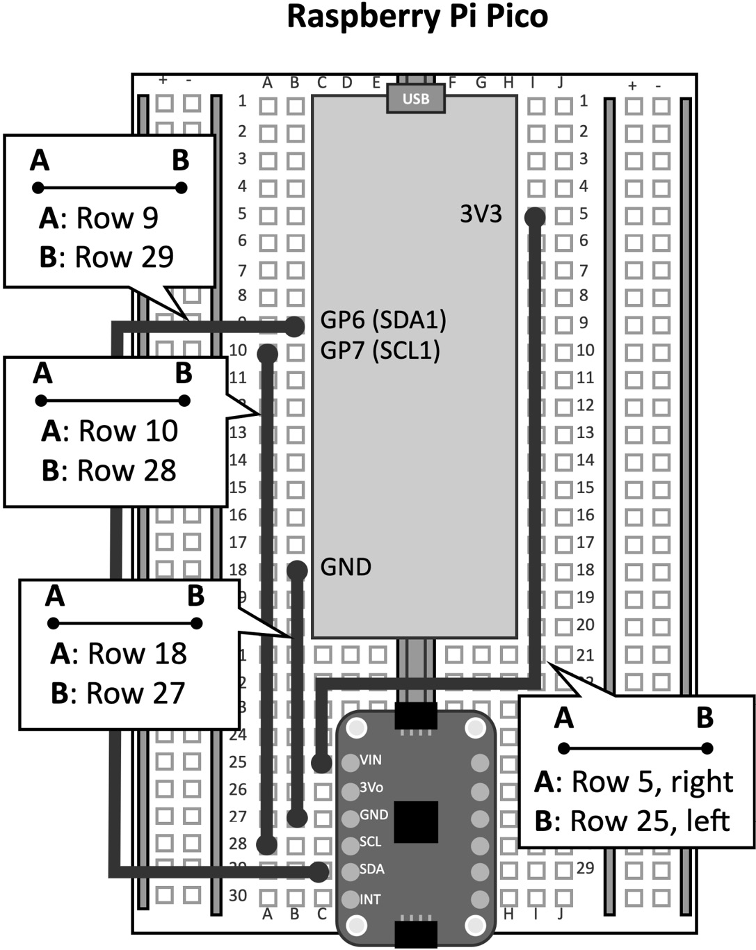
Figure 6.5 – Connections between the MPU-6050 IMU and Raspberry Pi Pico

As we mentioned in the Getting ready section of this recipe, we do not need pull-up resistors on SDA and SCL because they have already been integrated into the IMU's breakout board.

2. Create a new sketch in the Arduino IDE. Declare and initialize the mbed::I2C object with the SDA and SCL pins:

   #define I2C_SDA p6

   #define I2C_SCL p7

   I2C i2c(I2C_SDA, I2C_SCL);

The initialization of the I2C peripheral only requires the pins that are dedicated to the SDA (p6) and SCL (p7) buses.

3. Use a C define to keep the 7-bit address of the MPU-6050 IMU (0x68):

   #define MPU6050_ADDR_7BIT 0x68

Next, use a C define to keep the 8-bit address required that's for mbed::I2C. The 8-bit address can easily be obtained by left-shifting the 7-bit address by one bit:

#define MPU6050_ADDR_8BIT (0x68 << 1) //0xD1

4. Implement a utility function to read the data from an MPU-6050 register:

   void read_reg(int addr_i2c, int addr_reg, char *buf, int length) {

     char data = addr_reg;

     i2c.write(addr_i2c, &data, 1);

     i2c.read(addr_i2c, buf, length);

     return;

   }

As per the I2C protocol, we need to transmit the address of the MPU-6050 IMU and then send the address of the register to read. So, we must use the write() method of the mbed::I2C class, which needs three input arguments, as follows:

• The 8-bit address of the secondary device (addr_i2c)
• A char array containing the registered address (char data = addr_reg)
• The number of bytes to transmit (1 since we're only sending the registered address)

After sending the request to read the data from the register, we can get the data that's been transmitted by MPU-6050 with the read() method of the mbed::I2C class, which needs the following input arguments:

• The 8-bit address of the secondary device (addr_i2c)
• A char array to store the received data (buf)
• The size of the array (length)

The function will return once the read is complete.

5. In the setup() function, initialize the I2C frequency at the maximum speed that's supported by MPU-6050 (400 KHz):

   void setup() {

     i2c.frequency(400000);

6. In the setup() function, use read_reg() to read the WHO_AM_I register (0x75) of the MPU-6050 IMU. Transmit the MPU-6050 found message over the serial if the WHO_AM_I register contains the 7-bit device address (0x68):

     #define MPU6050_WHO_AM_I 0x75

     Serial.begin(115600);

     while(!Serial);

     char id;

     read_reg(MPU6050_ADDR_8BIT, MPU6050_WHO_AM_I, &id, 1);

     if(id == MPU6050_ADDR_7BIT) {

       Serial.println("MPU-6050 found");

     } else {

       Serial.println("MPU-6050 not found");

       while(1);

     }

   }

Compile and upload the sketch on the Raspberry Pi Pico. Now, you can open the serial Monitor from the Editor menu. If the Raspberry Pi Pico can communicate with the MPU-6050 device, it will transmit the MPU-6050 found string over serial.

Acquiring accelerometer data

The accelerometer is one of the most common sensors that's incorporated into the IMU.

In this recipe, we will develop an application to read the accelerometer measurements from the MPU-6050 IMU with a frequency of 50 Hz. The measurements will then be transmitted over the serial so that they can be acquired with the Edge Impulse data forwarder tool in the following recipe.

The following Arduino sketch contains the code that's referred to in this recipe

• 02_i2c_imu_read_acc.ino0:

https://github.com/PacktPublishing/TinyML-Cookbook/blob/main/Chapter06/ArduinoSketches/02_i2c_imu_read_acc.ino.

Getting ready

The accelerometer is a sensor that measures accelerations on one, two, or three spatial axes, denoted as X, Y, and Z.

In this and the following recipes, we will use the three-axis accelerometer that's integrated into the MPU-6050 IMU to measure the accelerations of three orthogonal directions.

However, how does the accelerometer work, and how can we take the measurements from the sensor?

Let's start by explaining the basic underlying working principle of this sensor. Consider the following system, which has a mass attached to a spring:

Figure 6.6 – Mass-spring system

The preceding diagram models the physical principle of an accelerometer working on a single spatial dimension (that is, a one-axis accelerometer).

What happens if we place the accelerometer on the table?

In this case, we will see the mass go down because of the constant gravitational force. Therefore, the lower spring on the Z-axis would have a displacement from the rest position, as shown in the following diagram:

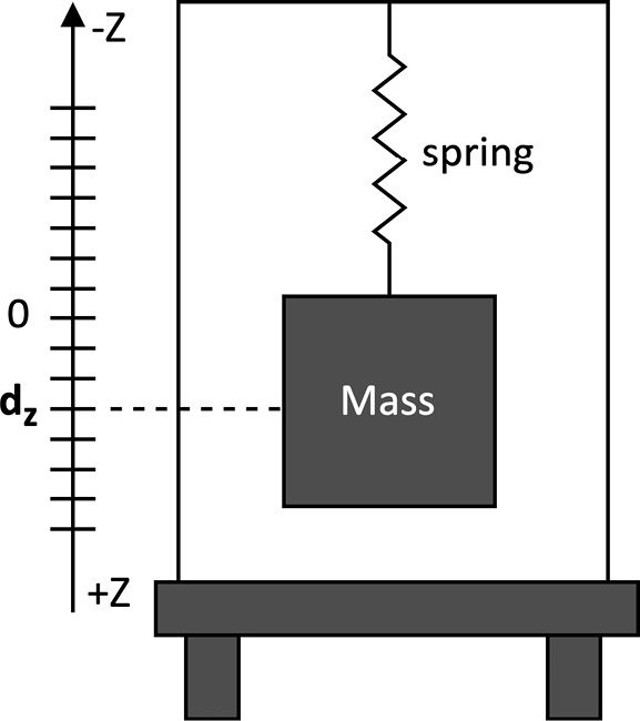
Figure 6.7 – The mass-spring system under the influence of gravitational force

From physics class, we know that Hooke's law gives the spring force (restoring force):

Here, is the force, is the elastic constant, and is the displacement.

From Newton's second law, we also know that the force that's applied on the mass is as follows:

Here, is the force, is the mass, and is the acceleration.

Under the constraint, we can infer that the spring displacement, , is proportional to the acceleration.

Hence, when a one-axis accelerometer is placed on the table, it returns ~9.81 m/s2, which is the object's acceleration when it's falling under the influence of gravity. The 9.81 m/s2 acceleration is commonly denoted with the g symbol (9.81 m/s2 = 1 g).

As we can imagine, the spring goes up and down whenever we move the accelerometer (even slightly). Therefore, the spring displacement is the physical quantity that's acquired by the sensor to measure acceleration.

An accelerometer that's working on two or three spatial dimensions can still be modeled with the mass-spring system. For example, a three-axis accelerometer can be modeled with three mass-spring systems so that each one returns the acceleration for a different axis.

Of course, we made some simplifications while explaining the device's functionality. Still, the core mechanism that's based on the mass-spring system is designed in silicon through the micro-electromechanical systems (MEMS) process technology.

Most accelerometers have a programmable measurement range (or scale) that can vary from ±1 g (±9.81 m/s2) to ±250 g (±2,452.5 m/s2). This range is also proportional to the sensitivity, which is commonly expressed as the least-significant bit over g (LSB/g) and defined as the minimum acceleration to cause a change in the numerical representation. Therefore, the higher the sensitivity, the smaller the minimum detectable acceleration.

In the MPU-6050 IMU, we can program the measurement range through the ACCEL_CONFIG register (0x1C). The following table reports the corresponding sensitivity for each one:

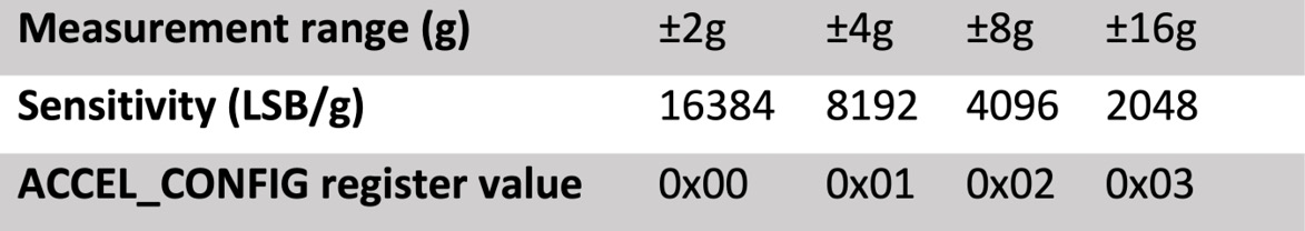
Figure 6.8 – Measurement range versus sensitivity on MPU-6050

As we can see, the smaller the measurement range, the higher the sensitivity. A ±2 g range is typically enough for acquiring accelerations due to hand movements.

The measurements that are returned by the MPU-6050 IMU are in 16-bit integer format and stored in two 8-bit registers. These two registers' names are marked with the _H and _L suffixes to identify the high and low bytes of the 16-bit variable. The following diagram shows the names and addresses of each register:

Figure 6.9 – Registers for the accelerometer measurements in the MPU-6050 IMU

As you can see, the registers are placed at consecutive memory addresses, starting with ACCEL_XOUT_H at 0x3B. To read all the accelerometer measurements without sending the address of each register, we can simply access ACCEL_XOUT_H and read 6 bytes.

How to do it…

Let's keep working on the sketch from the previous recipe. The following steps will show you how to extend the program to read accelerometer data from the MPU-6050 IMU and transmit the measurements over the serial:

1. Implement a utility function to write one byte into an MPU-6050 register:

   void write_reg(int addr_i2c, int addr_reg, char v) {

     char data[2] = {addr_reg, v};

     i2c.write(addr_i2c, data, 2);

     return;

   }

As shown in the preceding code, we use the write() method of the mbed::I2C class to transmit the following details:

1. The MPU-6050 address
2. The register address to access
3. The byte to store into the register

The write_reg() function will be required to initialize the MPU-6050 device.

2. Implement a utility function to read the accelerometer data from MPU-6050. To do so, create a function called read_accelerometer() with three input floating-point arrays:

   void read_accelerometer(float *x, float *y, float *z) {

The x, y, and z arrays will contain the sampled accelerations for the three orthogonal spatial directions.

3. In the read_accelerometer() function, read the accelerometer measurements from the MPU-6050 IMU:

     char data[6];

     #define MPU6050_ACCEL_XOUT_H 0x3B

     read_reg(MPU6050_ADDR_8BIT, MPU6050_ACCEL_XOUT_H, data, 6);

Next, combine the low and high byte of each measurement to get the 16-bit data format representation:

  int16_t ax_i16 = (int16_t)(data[0] << 8 | data[1]);

  int16_t ay_i16 = (int16_t)(data[2] << 8 | data[3]);

  int16_t az_i16 = (int16_t)(data[4] << 8 | data[5]);

Once you have these 16-bit values, divide the numbers by the sensitivity that's been assigned to the selected measurement range and multiply it by g (9.81 m/s2). Then, store the accelerations in the x, y, and z arrays:

  const float sensitivity = 16384.f;

  const float k = (1.f / sensitivity) * 9.81f;

  *x = (float)ax_i16 * k;

  *y = (float)ay_i16 * k;

  *z = (float)az_i16 * k;

  return;

}

The preceding code converts the raw data into an m/s2 numerical value. The sensitivity is 16384 because the MPU-6050 IMU will operate in the ±2 g range.

4. In the setup() function, ensure that the MPU-6050 IMU is not in sleep mode:

   #define MPU6050_PWR_MGMT_1 0x6B

   #define MPU6050_ACCEL_CONFIG 0x1C

   if (id == MPU6050_ADDR_7BIT) {

     Serial.println("MPU6050 found");

     write_reg(MPU6050_ADDR_8BIT, MPU6050_PWR_MGMT_1, 0);

When the IMU is in sleep mode, the sensor does not return any measurements. To ensure the MPU-6050 IMU is not in this operating mode, we need to clear the sixth bit (bit 6) of the PWR_MGMT_1 register. This can easily be done by clearing the PWR_MGMT_1 register directly.

5. In the setup() function, set the accelerometer measurement range of the MPU-6050 IMU to ±2 g:

     write_reg(MPU6050_ADDR_8BIT, MPU6050_ACCEL_CONFIG, 0);

   }

6. In the loop() function, sample the accelerometer measurements with a frequency of 50 Hz (50 three-axis accelerometer samples per second) and transmit them over the serial. Send the data with one line per accelerometer reading and the three-axis measurements (ax, ay, and az) comma-separated:

   #define FREQUENCY_HZ  50

   #define INTERVAL_MS   (1000 / (FREQUENCY_HZ + 1))

   #define INTERVAL_US   INTERVAL_MS * 1000

   void loop() {

     mbed::Timer timer;

     timer.start();

     float ax, ay, az;

     read_accelerometer(&ax, &ay, &az);

     Serial.print(ax);

     Serial.print(",");

     Serial.print(ay);

     Serial.print(",");

     Serial.println(az);

     timer.stop();

     using std::chrono::duration_cast;

     using std::chrono::microseconds;

     auto t0 = timer.elapsed_time();

     auto t_diff = duration_cast<microseconds>(t0);

     uint64_t t_wait_us = INTERVAL_US - t_diff.count();

     int32_t t_wait_ms = (t_wait_us / 1000);

     int32_t t_wait_leftover_us = (t_wait_us % 1000);

     delay(t_wait_ms);

     delayMicroseconds(t_wait_leftover_us);

   }

In the preceding code, we did the following:

1. Started the mbed::Timer before reading the accelerometer measurements to take the time required to acquire the samples.
2. Read the accelerations with the read_accelerometer() function.
3. Stopped mbed::Timer and retrieved the elapsed time in microseconds (µs).
4. Calculated how much time the program needs to wait before the next accelerometer reading. This step will guarantee the 50 Hz sampling rate.
5. Paused the program.

The program is paused with the delay() function, followed by delayMicroseconds(), due to the following reasons:

• delay() alone would be inaccurate since this timer needs the input argument in ms.
• delayMicroseconds() works up to 16 383 µs, which is insufficient for a sampling frequency of 50 Hz (2,000 µs).

So, we find out how much time to wait in milliseconds by dividing t_wait_us by 1,000. Then, we calculate the remaining time to wait in microseconds by calculating the remainder of the t_wait_us / 1000 division (t_wait_us % 1000).

The format that's used to send the accelerometer data over the serial (one line per reading with the three-axis measurements comma-separated) will be necessary to accomplish the task presented in the following recipe.

Compile and upload the sketch to the Raspberry Pi Pico. Next, open the serial monitor and check whether the microcontroller transmits the accelerometer measurements. If so, lay the breadboard flat on the table. The expected acceleration for the Z-axis (third number of each row) should be roughly equal to the acceleration due to gravity (9.81 m/s2), while the accelerations for the other axes should be approximately close to zero, as shown in the following diagram:

Figure 6.10 – Accelerations displayed in the Arduino serial monitor

As you can see, the accelerations could be affected by offset and noise. However, we don't need to worry about the accuracy of the measurements because the deep learning model will be capable of recognizing our gestures.

Building the dataset with the Edge Impulse data forwarder tool

Any ML algorithm needs a dataset, and for us, this means getting data samples from the accelerometer.

Recording accelerometer data is not as difficult as it may seem at first glance. This task can easily be carried out with Edge Impulse.

In this recipe, we will use the Edge Impulse data forwarder tool to take the accelerometer measurements when we make the following three movements with the breadboard:

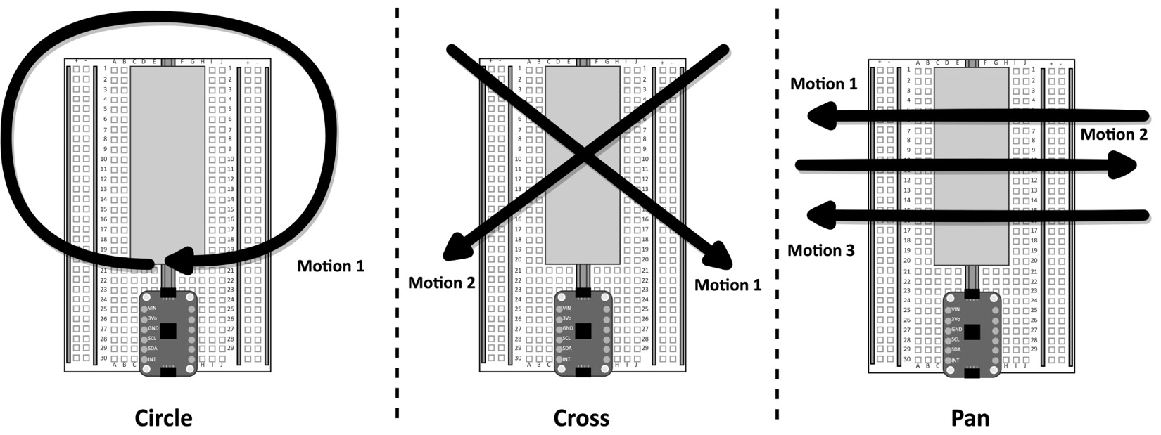
Figure 6.11 – Gestures to recognize – circle, cross, and pan

As shown in the preceding diagram, we should ensure that the breadboard is vertical, have our Raspberry Pi Pico in front of us, and make the movements that are shown by the arrows.

Getting ready

An adequate dataset for gesture recognition requires at least 50 samples for each output class. The three gestures that we've considered for this project are as follows:

• Circle: For moving the board clockwise in a circular motion.
• Cross: For moving the board from the top left to the bottom right and then from the right top to the bottom left.
• Pan: For moving the board horizontally to the left, then right, and then left again.

Each gesture should be performed by placing the breadboard vertically and with the Raspberry Pi Pico in front of us. Since we will consider training samples with a duration of 2.5 seconds, we recommend completing each movement in roughly 2 seconds.

Although we have three output classes to identify, an additional one is required to cope with the unknown movements and the case where there are no gestures (for example, the breadboard lying flat on the table).

In this recipe, we will use the Edge Impulse data forwarder to build our dataset. This tool allows us to quickly acquire the accelerations from any device that's capable of transmitting data over the serial and import the sample directly in Edge Impulse.

The data forwarder will run on your computer, so you will need to have the Edge Impulse CLI installed. If you haven't installed the Edge Impulse CLI yet, we recommend following the instructions in the official documentation: https://docs.edgeimpulse.com/docs/cli-installation.

How to do it…

Compile and upload the sketch that we developed in the previous recipe on your Raspberry Pi Pico. Ensure the Arduino serial monitor is closed; the serial peripheral on your computer can only communicate with one application at a time.

Next, open Edge Impulse and create a new project. Edge Impulse will ask you to write the name of the project. In our case, we have named the project gesture_recognition.

Now, follow these steps to build the dataset with the data forwarder tool:

1. Run the edge-impulse-data-forwarder program on your computer with a 50 Hz frequency and 115600 baud rate:

   $ edge-impulse-data-forwarder -- frequency 50 --baud-rate 115600

The data forwarder will ask you to authenticate on Edge Impulse, select the project you are working on, and give your Raspberry Pi Pico a name (for example, you can call it pico).

Once you have configured the tool, the program will start parsing the data that's being transmitted over the serial. The data forwarder protocol expects one line per sensor reading with the three-axis accelerations either comma (,) or tab separated, as shown in the following diagram:

Figure 6.12 – Data forwarder protocol

Since our Arduino sketch complies with the protocol we just described, the data forwarder will detect the three-axis measurements that are being transmitted over the serial and ask you to assign a name. You can call them ax, ay, and az.

2. Open Edge Impulse and click on the Data acquisition tab from the left-hand side menu.

As shown in the following screenshot, use the Record new data area to record 50 samples for each gesture (circle, cross, and pan):

Figure 6.13 – The Record new data window in Edge Impulse

The Device and Frequency fields should already report the name of the device that's connected to the data forwarder (pico), as well as the sampling frequency (50Hz).

For each gesture, enter the label's name in the Label field (for example, circle for the circle gesture) and the duration of the recording in Sample length (ms.).

Although each sample has a duration of 2.5 seconds, you can conveniently acquire 20 seconds of data where you repeat the same gestures multiple times, as shown in the following screenshot:

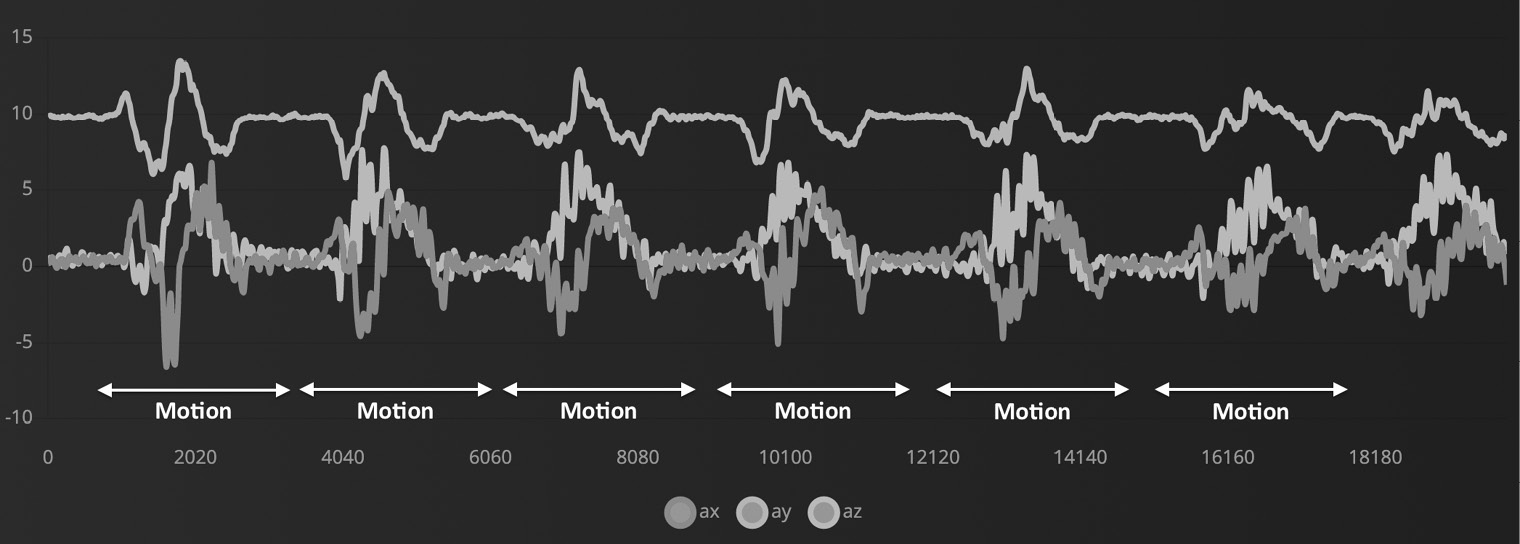
Figure 6.14 – A single recording with multiple motions of the same type

However, we recommend waiting 1 or 2 seconds between movements to help Edge Impulse recognize the motions in the following step.

3. Split the recording into samples of 2.5 seconds by clicking on near the filename and then clicking Split sample, as shown in the following screenshot:

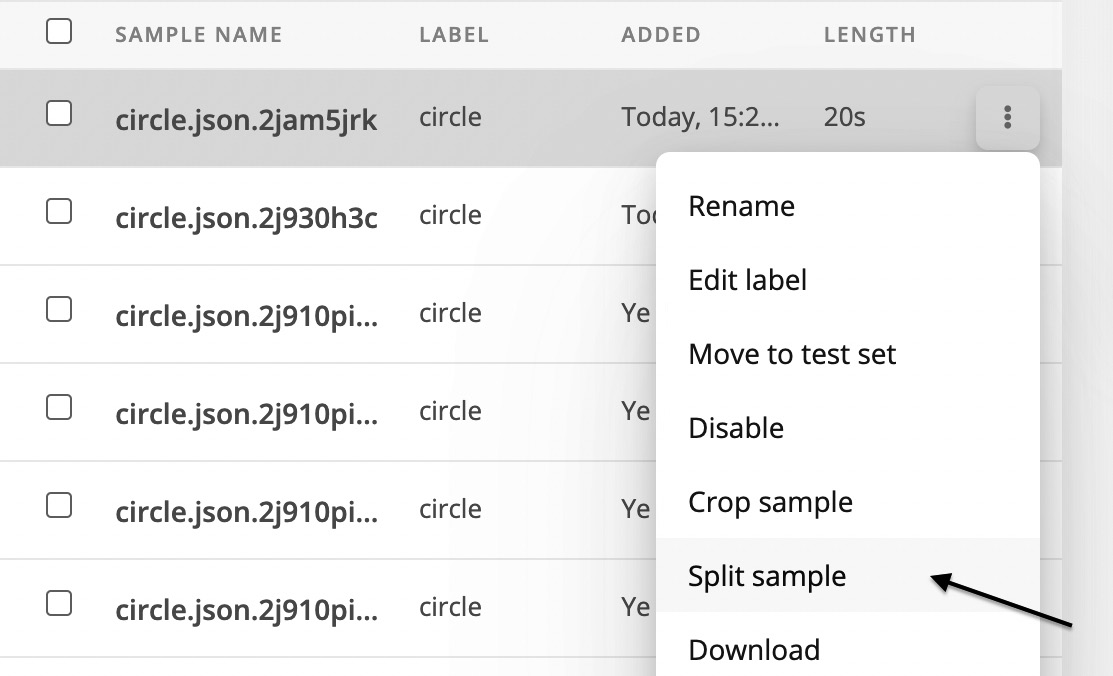
Figure 6.15 – The Split sample option in Edge Impulse

Set segment length (ms.) to 2500 (2.5s) in the new window and click Apply. Edge Impulse will detect the motions and put a cutting window of 2.5 seconds on each one, as shown in the following screenshot:

Figure 6.16 – Sample splits in windows of 2.5 seconds

If Edge Impulse does not recognize a motion in the recording, you can always add the window manually by clicking the Add Segment button and clicking on the area you want to cut.

Once all the segments have been selected, click Split to get the individual samples.

4. Use the Record new data area to record 50 random motions for the unknown class. To do so, acquire 40 seconds of accelerometer data where you move the breadboard randomly and lay it flat on the table.
5. Split the unknown recording into samples of 2.5 seconds by clicking on near the filename and then Split sample. In the new window, add 50 cutting windows and click on Split when you are done.
6. Split the samples between the training and test datasets by clicking on the Perform train/test split button in the Danger zone area of the dashboard.

Edge Impulse will ask you twice if you are sure that you want to perform this action. This is because the data shuffling operation is irreversible.

The dataset is now ready, with 80% of the samples assigned to the training/validation set and 20% to the test set.

Designing and training the ML model

With the dataset in our hands, we can start designing the model.

In this recipe, we will develop the following architecture with Edge Impulse:

Figure 6.17 – Fully connected neural network to train

As you can see, the spectral features are the input for the model, which consists of just two fully connected layers.

Getting ready

In this recipe, we want to explain why the tiny network shown in the preceding diagram recognizes gestures from accelerometer data.

When developing deep neural network architectures, we commonly feed the model with raw data to leave the network to learn how to extract the features automatically.

This approach proved to be effective and incredibly accurate in various applications, such as image classification. However, there are some applications where hand-crafted engineering features offer similar accuracy results to deep learning and help reduce the architecture's complexity. This is the case for gesture recognition, where we can use features from the frequency domain.

Note

If you are not familiar with frequency domain analysis, we recommend reading Chapter 4, Voice Controlling LEDs with Edge Impulse.

The benefits of spectral features will be described in more detail in the following subsection.

Using spectral analysis to recognize gestures

Spectral analysis allows us to discover characteristics of the signal that are not visible in the time domain. For example, consider the following two signals:

Figure 6.18 – Two signals in the time domain

These two signals are assigned to two different classes: class 0 and class 1.

What features would you use in the time domain to discriminate class 0 from class 1?

Whatever set of features you may consider, they must be shift-invariant and robust to noise to be effective. Although there may be a set of features to distinguish class 0 from class 1, the solution would be straightforward if we considered the problem in the frequency domain, as shown by their power spectrums in the following diagram:

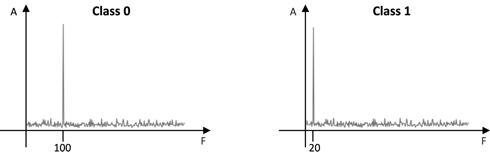
Figure 6.19 – Frequency representations of the class 0 and class 1 signals

As we can see, the two signals have different dominant frequencies, defined as the components with the highest magnitude. In other words, the dominant frequencies are the components that carry more energy.

Although signals from an accelerometer are not the same as class 0 and class 1, they still have repetitive patterns that make the frequency components suitable for a classification problem.

However, the frequency representation also offers another benefit related to the possibility of getting a compressed representation of the original signal.

For example, let's consider our dataset samples, which are three-axis accelerations that we acquired with a frequency of 50 Hz for 2.5 seconds. Each instance contains 375 data points (125 data points per axis). Now, let's apply the Fast Fourier Transform (FFT) with 128 output frequencies (FFT length) on each sample. This domain transformation produces 384 data points (128 data points per axis). Hence, FFT appears to be reducing the amount of data. However, as we saw in the previous example with class 0 and class 1, not all frequencies bring meaningful information. Therefore, we could just extract the frequencies that get the most energy (dominant frequencies) to reduce the amount of data and then facilitate signal pattern recognition.

For gesture recognition, we commonly produce spectral features by doing the following:

1. Applying a low-pass filter to the frequency domain to filter out the highest frequencies. This step generally makes feature extraction more robust against noise.
2. Extracting the frequency components with the highest magnitude. Commonly, we take the three frequencies with the highest peak.
3. Extracting the power features in the power spectrum. Generally, these features are the root mean square (RMS) and the power spectral density (PSD), which describe the power that's present in an interval of frequencies.

In our case, we will extract the following features for each accelerometer axis:

• One value for the RMS
• Six values for extracting the frequencies with the highest peak (three values for the frequency and three values for the magnitude)
• Four values for the PSD

Therefore, we would only get 33 features, which means a data reduction of over 11 times compared to the original signal, which is enough to feed a tiny fully connected neural network.

How to do it…

Click on the Create Impulse tab from the left-hand side menu. In the Create Impulse section, set Window size to 2500ms and Window increase to 200ms.

As we saw in Chapter 4, Voice Controlling LEDs with Edge Impulse, the Window increase parameter is required to run ML inference at regular intervals. This parameter plays a crucial role in a continuous data stream since we do not know when the event may start. Therefore, the idea is to split the input data stream into fixed windows (or segments) and execute the ML inference on each one. Window size is the temporal length of the window, while Window increase is the temporal distance between two consecutive segments.

The following steps will show how to design the neural network shown in Figure 6.17:

1. Click the Add a processing block button and look for Spectral Analysis:

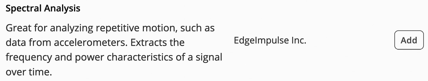
Figure 6.20 – The Spectral Analysis processing block

Click the Add button to integrate the processing block into Impulse.

2. Click the Add a learning block button and add Classification (Keras).

Output features block should report the four output classes we must recognize (circle, cross, pan, and unknown), as shown in the following screenshot:

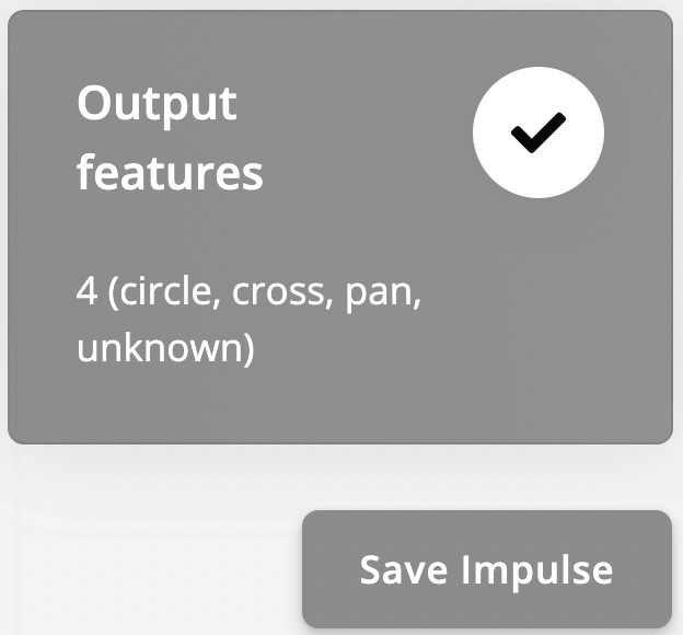
Figure 6.21 – Output classes

Save the Impulse by clicking the Save Impulse button.

3. Click on the Spectral features button from the Impulse design category:

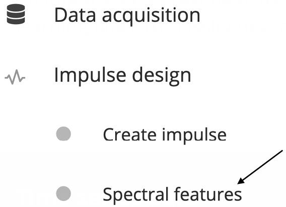
Figure 6.22 – Spectral features button

In the new window, we can play with the parameters that are affecting the feature extraction, such as the following:

• The type of filter to apply to the input signal: We can either select a low-pass or high-pass filter and then set the cut-off frequency, the frequency at which attenuation occurs due to the filter increasing rapidly. Since we want to filter out the contribution of the noise, we should use a low-pass filter.
• The parameters that are affecting the spectral power features being extracted: This includes the FFT length, the number of frequency components with the highest peak to extract, and the power edges that are required for the PSD.

We can keep all the parameters at their default values and click on the Generate features button to extract the spectral features from each training sample. Edge Impulse will return the Job completed message in the output log when the feature extraction process ends.

4. Click on the Neural Network (Keras) button under the Impulse design section and add a Dropout layer with a 0.2 ratio between the fully connected layers. Ensure that the first fully connected layer has 33 neurons while the other has 10 neurons, as shown in the following screenshot:

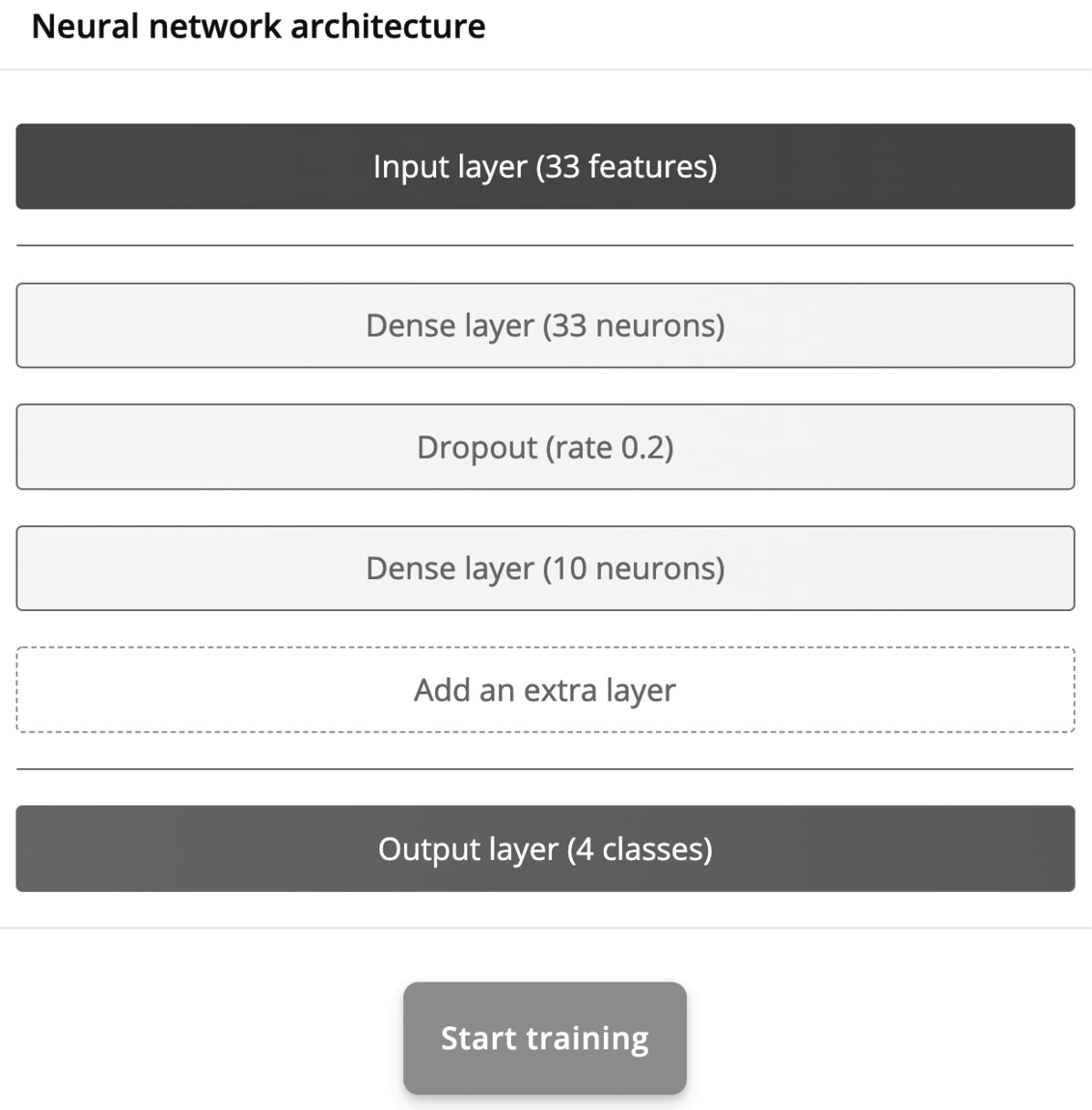
Figure 6.23 – Neural network architecture

Set the number of training epochs to 100 and click on Start training.

The output console will report the accuracy and loss on the training and validation datasets during training after each epoch.

Now, let's evaluate the model's performance on the test dataset. To do so, click the Model testing button from the left panel and then click Classify all.

Edge Impulse will provide this progress in Model testing output and generate the confusion matrix once the process is completed:

Figure 6.24 – Model testing results

As you can see, our tiny model, which is made up of just two fully connected layers, achieved 88% accuracy!

Live classifications with the Edge Impulse data forwarder tool

Model testing is the step we should always take before exporting the final application to the target platform. Deploying on microcontrollers is error-prone because the code may contain bugs, the integration could be incorrect, or the model could not work reliably in the field. Therefore, model testing is necessary to exclude at least ML from the source of failures.

In this recipe, we will learn how to perform live classifications via Edge Impulse using the Raspberry Pi Pico.

Getting ready

The most effective way to evaluate the behavior of an ML model is to test the model's performance on the target platform.

In our case, we have already got a head start because the dataset was built with the Raspberry Pi Pico. Therefore, the accuracy of the test dataset should already give us a clear indication of how the model behaves. However, there are cases where the dataset may not be built on top of sensor data coming from the target device. When this happens, the model that's been deployed on the microcontroller could behave differently from what we expect. Usually, the reason for this performance degradation is due to sensor specifications. Fundamentally, sensors can be of the same type but have different specifications, such as offset, accuracy, range, sensitivity, and so on.

Thanks to the Edge Impulse data forwarder tool, it is straightforward to discover how the model performs on our target platform.

How to do it…

Ensure your Raspberry Pi Pico is still running the program we developed in the Acquiring accelerometer data recipe and that the edge-impulse-data-forwarder program is running on your computer. Next, click the Live classification tab and check whether the device (for example, pico) is being reported in the Device drop-down list, as shown in the following screenshot:

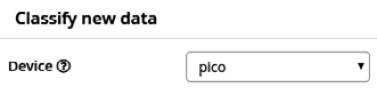
Figure 6.25 – The Device dropdown menu in Edge Impulse

If the device is not listed, follow the steps provided in the How to do it… subsection of the Acquiring accelerometer data recipe to pair your Raspberry Pi Pico with Edge Impulse again.

Now, follow these steps to evaluate the model's performance with the live classification tool:

1. In the Live classification window, select Sensor with 3 axes from the Sensor drop-down list and set Sample length (ms) to 20000. Keep Frequency at the default value (50 Hz).
2. With your Raspberry Pi Pico in front of you, click Start sampling and wait for the Sampling… message to appear on the button.

When the recording begins, make any of the three movements that the model can recognize (circle, cross, or pan). The sample will be uploaded to Edge Impulse when the recording ends.

Edge Impulse will then split the recording into samples of 2.5 seconds and test the trained model on each. The classification results will be reported on the same page, similar to what we saw in Chapter 4, Voice Controlling LEDs with Edge Impulse.

Gesture recognition on Raspberry Pi Pico with Arm Mbed OS

Now that the model is ready, we can deploy it on the Raspberry Pi Pico.

In this recipe, we will build a continuous gesture recognition application with the help of Edge Impulse, Arm Mbed OS, and an algorithm to filter out redundant or spurious classification results.

The following Arduino sketch contains the code that will be referred to in this recipe:

• 06_gesture_recognition.ino:

https://github.com/PacktPublishing/TinyML-Cookbook/blob/main/Chapter06/ArduinoSketches/06_gesture_recognition.ino.

Getting ready

In this recipe, we will make our Raspberry Pi Pico capable of recognizing gestures with the help of the library that's generated by Edge Impulse for Arduino IDE. In Chapter 4, Voice Controlling LEDs with Edge Impulse, we used a pre-built example to accomplish this. However, here, we will implement the entire program from scratch.

Our goal is to develop a continuous gesture recognition application, which means that the accelerometer data sampling and ML inference must be performed concurrently. This approach guarantees that we capture and process all the pieces of the input data stream so that we don't miss any events.

The main ingredients we will need to accomplish our task are as follows:

• Arm Mbed OS for writing a multithreading program
• An algorithm to filter out redundant classification results

Let's start by learning how to perform concurrent tasks easily with the help of real-time operating system (RTOS) APIs in Arm Mbed OS.

Creating working threads with RTOS APIs in Arm Mbed OS

Any Arduino sketches that have been developed for the Arduino Nano 33 BLE Sense board and Raspberry Pi Pico are built on top of Arm Mbed OS, an open source RTOS for Arm Cortex-M microcontrollers. So far, we have only used Mbed APIs for interfacing with peripherals such as GPIO and I2C. However, Arm Mbed OS also offers functionalities that are typical of a canonical OS, such as managing threads to perform different tasks concurrently.

Once the thread has been created, we just need to bind the thread to the function that we want to run and execute it when we are ready.

Tip

If you are interested in learning more about the functionalities of Arm Mbed OS, we recommend reading the official documentation, which can be found at the following link: https://os.mbed.com/docs/mbed-os/v6.15/bare-metal/index.html.

A thread in a microcontroller is a piece of a program that runs independently on a single core. Since all the threads run on the same core, the scheduler is responsible for deciding on what to execute and for how long. Mbed OS uses a pre-emptive scheduler and uses a round-robin priority-based scheduling algorithm (https://en.wikipedia.org/wiki/Round-robin_scheduling). Therefore, every thread is assigned to a priority that's provided by us when we create the thread object through the RTOS API of Mbed OS (https://os.mbed.com/docs/mbed-os/v6.15/apis/thread.html). The supported priority values can be found at https://os.mbed.com/docs/mbed-os/v6.15/apis/thread.html.

For this recipe, we will need two threads:

• Sampling thread: The thread that's responsible for acquiring the accelerations from the MPU-6050 IMU with a frequency of 50 Hz
• Inference thread: The thread that's responsible for running model inference after every 200 ms

However, as we mentioned at the beginning of this Getting ready section, a multithreading program is not the only ingredient that's required to build our gesture recognition application. A filtering algorithm will also be necessary to filter out redundant and spurious predictions.

Filtering out redundant and spurious predictions

Our gesture recognition application employs a sliding window-based approach over a continuous data stream to determine whether we have a motion of interest. The idea behind this approach is to split the data stream into smaller windows of a fixed size and execute the ML inference on each one.. As we already know, ML is a powerful tool for gathering robust classification results, especially if we use temporal shifts on the input data. Therefore, neighboring windows will have similar and high probability scores, leading to multiple and redundant detections.

In this recipe, we will adopt a test and trace filtering algorithm to make our application robust against spurious detections. Conceptually, this filtering algorithm only wants to consider the ML output class as valid if the last N predictions (for example, the last four) reported the following:

• The same output class but it's different from the unknown one.
• The probability score is above a fixed threshold (for example, greater than 0.7).

To visually understand how this algorithm works, look at the following diagram:

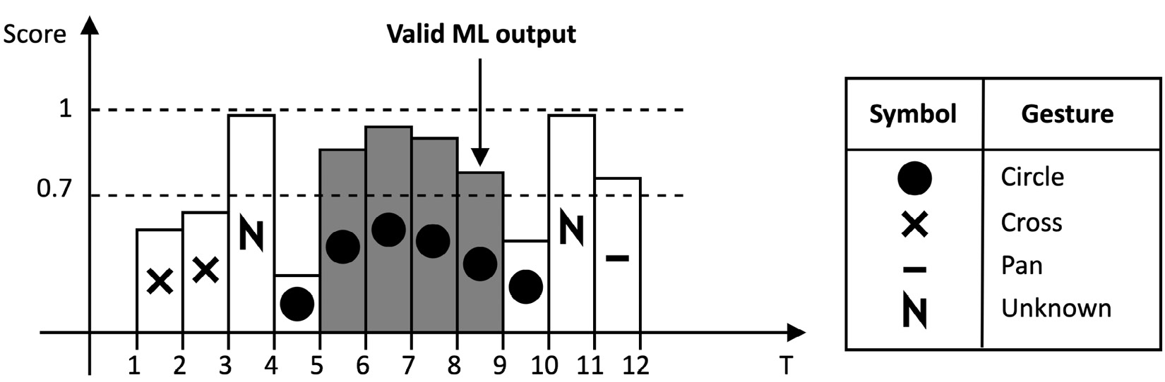
Figure 6.26 – Example of a valid ML prediction

In the preceding diagram, each rectangular bar is the predicted class at a given time, where the following occurs:

• The symbol represents the predicted output class
• The bar's height is the probability score associated with the predicted class

Therefore, considering N as four and the probability threshold as 0.7, we can consider the ML output class as valid only at T=8. The previous four classification results returned circle and had probability scores greater than 0.7.

How to do it…

Click on Deployment from the left-hand side menu and select Arduino Library from the Create library options, as shown in the following screenshot:

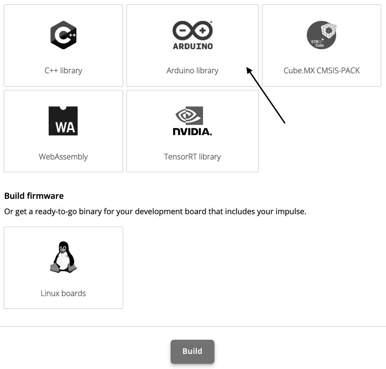
Figure 6.27 – Edge Impulse deployment section

Then, click on the Build button at the bottom of the page. Save the ZIP file on your computer.

Next, import the library into the Arduino IDE. After that, copy the sketch that we developed in the Acquiring accelerometer data recipe in a new sketch. Follow these steps to learn how to extend this code to make the Raspberry Pi Pico capable of recognizing our three gestures:

1. Include the <edge_impulse_project_name>_inferencing.h header file in the sketch. For example, if the Edge Impulse project's name is gesture_recognition, you should include the following information:

   #include <gesture_recognition_inferencing.h>

This header file is the only requirement for using the constants, functions, and C macros that have been built by Edge Impulse specifically for our project.

2. Declare two floating-point arrays (buf_sampling and buf_inference) that have 375 elements each:

   #define INPUT_SIZE EI_CLASSIFIER_DSP_INPUT_FRAME_SIZE

   float buf_sampling[INPUT_SIZE] = { 0 };

   float buf_inference[INPUT_SIZE];

In the preceding code, we used the Edge Impulse EI_CLASSIFIER_DSP_INPUT_FRAME_SIZE C macro definition to get the number of input samples that are required for 2.5 seconds of accelerometer data (375).

The buf_sampling array will be used by the sampling thread to store the accelerometer data, while the buf_inference array will be used by the inference thread to feed the input to the model.

3. Declare an RTOS thread with a low priority schedule for running the ML model:

   rtos::Thread inference_thread(osPriorityLow);

The inference thread should have a lower priority (osPriorityLow) than the sampling thread because it has a longer execution time due to ML inference. Therefore, a low priority schedule for the inference thread will guarantee that we do not miss any accelerometer data samples.

4. Create a C++ class to implement the test and trace filtering algorithm. Make the filtering parameters (N and probability threshold) and the variables that are needed to trace the ML predictions (counter and the last output valid class index) as private members:

   class TestAndTraceFilter {

   private:

     int32_t       _n {0};

     float         _thr {0.0f};

     int32_t       _counter {0};

     int32_t       _last_idx_class {-1};

     const int32_t _num_classes {3};

The algorithm mainly needs two variables to trace the classification results. These variables are as follows:

• _counter: This variable is used to keep track of how many times we had the same classification with a probability score above the fixed threshold (_thr).
• _last_idx_class: This variable is used to find the output class index of the last inference.

In this recipe, we will assign -1 to the _last_idx_class variable when the last inference returns either unknown or a probability score below the fixed threshold (_thr).

5. Declare the invalid output index class (-1) as a public member:

   public:

     static constexpr int32_t invalid_idx_class = -1;

6. Implement the TestAndTraceFilter constructor to initialize the filtering parameters:

   public:

     TestAndTraceFilter(int32_t n, float thr) {

       _thr = thr;

       _n   = n;

     }

7. In the TestAndTraceFilter class, implement a private method to reset the internal variables (_counter and _last_idx_class) that will be used to trace the ML predictions:

     void reset() {

       _counter        = 0;

       _last_idx_class = invalid_idx_class;

     }  

8. In the TestAndTraceFilter class, implement a public method to update the filtering algorithm with the latest classification result:

     void update(size_t idx_class, float prob) {

       if(idx_class >= _num_classes || prob < _thr) {    

         reset();

       }

       else {

         if(prob > _thr) {

           if(idx_class != _last_idx_class) {

             _last_idx_class = idx_class;

             _counter        = 0;

           }

           _counter += 1;

         }

         else {

           reset();

         }

       }

     }  

The TestAndTraceFilter object works in two states – incremental and reset – as shown in the following diagram:

Figure 6.28 – Test and trace filtering flowchart

As you can see, the incremental state occurs when the most recent classification is a valid output class and the probability is greater than the minimum probability value. In all the other cases, we enter the reset state, where we set _counter to 0 and _last_idx_class to -1.

In the incremental state, _counter is incremented by one, and _last_idx_class keeps the index of the valid output class.

9. In the TestAndTraceFilter class, implement a public method to return the filter's output:

     int32_t output() {

       if(_counter >= _n) {

         int32_t out = _last_idx_class;

         reset();

         return out;

       }

       else {

         return invalid_idx_class;

       }

     }  

As you can see, if _counter is greater than or equal to _n, we return _last_idx_class and put the test and trace filter function in the reset state.

If _counter is smaller than _n, we return invalid_idx_class.

10. Write a function to run the ML inference (inference_func) in an infinite loop (while(1)). This function will be executed by the RTOS thread (inference_thread). Before you start this inference, wait for the sampling buffer to become full:

    void inference_func() {

      delay((EI_CLASSIFIER_INTERVAL_MS * EI_CLASSIFIER_RAW_SAMPLE_COUNT) + 100);

Next, initialize the test and trace filter object. Set N and probability threshold to 4 and 0.7f, respectively:

  TestAndTraceFilter filter(4, 0.7f);

After the initialization, run the ML inference in an infinite loop:

  while (1) {

    memcpy(buf_inference, buf_sampling,

           INPUT_SIZE * sizeof(float));

    signal_t signal;

    numpy::signal_from_buffer(buf_inference, INPUT_SIZE,

                              &signal);

    ei_impulse_result_t result = { 0 };

    run_classifier(&signal, &result, false);

Before we run the inference, we need to copy the data from buf_sampling to buf_inference and initialize the Edge Impulse signal_t object with the buf_inference buffer.

11. Get the output class with the highest probability and update the TestAndTraceFilter object with the latest classification result:

        size_t ix_max = 0; float  pb_max = 0;

    #define NUM_OUTPUT_CLASSES EI_CLASSIFIER_LABEL_COUNT

        for (size_t ix = 0; ix < NUM_OUTPUT_CLASSES; ix++) {

          if(result.classification[ix].value > pb_max) {

            ix_max = ix;

            pb_max = result.classification[ix].value;

          }

        }

        filter.update(ix_max, pb_max);

12. Read the output of the TestAndTraceFilter object. If the output is not -1 (invalid output), send the label that was assigned to the predicted gesture over the serial:

        int32_t out = filter.output();

        if(out != filter.invalid_idx_class) {

          Serial.println(result.classification[out].label);

        }

Next, wait for 200 ms (window increase set in the Edge Impulse project) before running the subsequent inference:

    delay(200);

Note

delay() puts the current thread in a waiting state. As a rule of thumb, we should always put a thread in a waiting state when it does not perform computation for a long time. This approach guarantees that we don't waste computational resources and that other threads can run in the meantime.

13. Start the RTOS inference thread (inference_thread) in the setup() function:

    inference_thread.start(mbed::callback(&inference_func));

14. In the loop() function, replace the prints to the serial port with the code that's required to store the accelerometer measurements in buf_sampling:

      float ax, ay, az;

      read_accelerometer(&ax, &ay, &az);

      numpy::roll(buf_sampling, INPUT_ SIZE, -3);

      buf_sampling[INPUT_SIZE - 3] = ax;

      buf_sampling[INPUT_SIZE - 2] = ay;

      buf_sampling[INPUT_SIZE - 1] = az;

Since the Arduino loop() function is an RTOS thread with high priority, we don't need to create an additional thread to sample the accelerometer measurements. Therefore, we can replace the Serial.print functions with the code that's required to fill the buf_sampling buffer with the accelerometer data.

The buf_sampling buffer is filled as follows:

• First, we shift the data in the buf_sampling array by three positions using the numpy::roll() function. The numpy::roll() function is provided by the Edge Impulse library, and it works similarly to its NumPy counterpart. (https://numpy.org/doc/stable/reference/generated/numpy.roll.html).
• Then, we store the three-axis accelerometer measurements (ax, ay, and az) in the last three positions of buf_sampling.

This approach will ensure that the latest accelerometer measurements are always in the last three positions of buf_sampling. By doing this, the inference thread can copy this buffer's content into the buf_inference buffer and feed the ML model directly without having to perform data reshuffling.

Compile and upload the sketch on the Raspberry Pi Pico. Now, if you make any of the three movements that the ML model can recognize (circle, cross, or pan), you will see the recognized gestures in the Arduino serial terminal.

Building a gesture-based interface with PyAutoGUI

Now that we can recognize the hand gestures with the Raspberry Pi Pico, we must build a touchless interface for YouTube video playback.

In this recipe, we will implement a Python script to read the recognized motion that's transmitted over the serial and use the PyAutoGUI library to build a gesture-based interface to play, pause, mute, unmute, and change YouTube videos.

The following Python script contains the code that's referred to in this recipe:

• 07_gesture_based_ui.py:

https://github.com/PacktPublishing/TinyML-Cookbook/blob/main/Chapter06/PythonScripts/07_gesture_based_ui.py.

Getting ready

The Python script that we will develop in this recipe will not be implemented in Google Colaboratory because that requires accessing the local serial port, keyboard, and monitor. Therefore, we will write the program in a local Python development environment.

We only need two libraries to build our gesture-based interface: pySerial and PyAutoGUI.

PySerial will be used to grab the predicted gesture that will be transmitted over serial, similar to what we saw in Chapter 5, Indoor Scene Classification with TensorFlow Lite for Microcontrollers and the Arduino Nano.

The identified movement, in turn, will perform one of the following three YouTube video playback actions:

Figure 6.29 – Table reporting the gesture mapping

Since YouTube offers keyboard shortcuts for the preceding actions (https://support.google.com/youtube/answer/7631406), we will use PyAutoGUI to simulate the keyboard keys (keystrokes) that are pressed, as shown in the following table:

Figure 6.30 – Keyboard shortcuts for the YouTube playback actions

For example, if the microcontroller returns circle over the serial, we will need to simulate the press of the m key.

How to do it…

Ensure you have installed PyAutoGUI in your local Python development environment (for example, pip install pyautogui). After that, create a new Python script and import the following libraries:

import serial

import pyautogui

Now, follow these steps to build a touchless interface with PyAutoGUI:

1. Initialize pySerial with the port and baud rate that's used by the Raspberry Pi Pico::

   port = '/dev/ttyACM0'

   baudrate = 115600

   ser = serial.Serial()

   ser.port     = port

   ser.baudrate = baudrate

Once initialized, open the serial port and discard the content in the serial input buffer:

ser.open()

ser.reset_input_buffer()

2. Create a utility function to return a line from the serial port as a string:

   def serial_readline():

     data = ser.readline

     return data.decode("utf-8").strip()

3. Use a while loop to read the serial data line by line:

   while True:

     data_str = serial_readline()

For each line, check whether we have a circle, cross, or pan motion.

If we have a circle motion, press the m key to mute/unmute:

if str(data_str) == "circle":  

  pyautogui.press('m')

If we have a cross motion, press the k key to play/pause:

if str(data_str) == "cross":  

  pyautogui.press('k')

If we have a pan motion, press the Shift + N hotkey to move to the next video:

if str(data_str) == "pan":  

  pyautogui.hotkey('shift', 'n')

4. Start the Python script while ensuring your Raspberry Pi Pico is running the sketch that we developed in the previous recipe.

Next, open YouTube from your web browser, play a video, and have your Raspberry Pi Pico in front of you. Now, if you make any of the three movements that the ML model can recognize (circle, cross, or pan), you will be able to control the YouTube video playback with gestures!